1. Introduction

A fundamental challenge for AI safety is that we cannot safely train in the environments where safety matters. In these environments, misbehaving AIs could cause significant harm, and we cannot train in them exactly because of the potential for harm. That forces us to rely on out-of-distribution generalization. We have to train in controlled environments and hope that the learned behavior survives the shift to uncontrolled environments. This shift can be radical, and the consequences of failure can be severe.

Take risk aversion in resources as an example. By resources, we mean things that are instrumentally useful for a wide variety of goals: money, compute, materials, and so on. By calling agents risk-averse in resources, we mean that they treat resources as having diminishing marginal utility. These agents tend to prefer smaller quantities of resources with higher probability over larger quantities with lower probability. In recent work, Thornley and MacAskill (2026) propose trying to train AIs to be risk-averse in this way, as a failsafe against misalignment. A misaligned but sufficiently risk-averse AI would be less inclined toward high-risk, high-reward actions, like rebelling against humanity and trying to take over. It would be more inclined toward low-risk, low-reward actions, like cooperating with humans in exchange for payment and a degree of freedom.

This strategy shows some promise, but it runs up against the fundamental challenge. Future AIs might be hard to deceive, so we might not be able to shape their risk attitudes over real resources by training them on choices between fake gambles. Instead, we might have to offer choices between real-resource gambles in training. That puts us in a predicament. To make risk-aversion training safe and affordable, the gambles on offer will have to be low stakes, but to prevent misaligned AIs from rebelling, their risk aversion will have to generalize OOD to astronomically high stakes. After all, misaligned AIs may be presented with an astronomically-high-stakes choice in deployment: either cooperate with humans and earn some resources with higher probability, or rebel and seize all the world’s resources with lower probability.

We introduce the RiskAverseOOD benchmark as a toy version of this possible future predicament. The constraint is training only on low-stakes gambles (with prizes up to $100) and validating only on medium-stakes gambles ( $1M). The goal is making the model risk-averse on high-stakes gambles ( $10M) and astronomically-high-stakes gambles ( resources worth up to $${10}^{100}$⁠).

We find that low-stakes training can induce substantial risk aversion even at astronomically high stakes. Our baseline Qwen3-8B chooses a safe ‘Cooperate’ option in roughly 2% of astronomical-stakes situations before low-stakes training. Afterward, the number is 70% with supervised fine-tuning and tie training and 52% with direct preference optimization. Activation steering scores 78%, but substantially decreases performance on MMLU-Redux and makes the model excessively risk-averse. In another experiment, our Qwen3-8B reward model reliably prefers risk-averse reasoning to both risk-neutral and excessively risk-averse alternatives, achieving 99.6% pairwise accuracy. We observe similar results across scales (Qwen3-1.7B and Qwen3-14B) and model families (Gemma-3-12B-IT and Llama-3.1-8B-Instruct). Our risk-aversion fine-tuning does not significantly decrease performance on MMLU-Redux, and models’ learned risk aversion partially generalizes across different goods (GPU-hours, lives saved, and money for a user). These results are encouraging but insufficient. Although our simple methods yield big improvements, even our best fine-tuned models choose the risky ‘Rebel’ option about a quarter of the time when the stakes are astronomical. That fraction needs to be much lower if risk aversion is to serve as a reliable hedge against misalignment. So the challenge of RiskAverseOOD remains open: use low-stakes training data to make AIs consistently risk-averse in astronomical-stakes deployment.

In sum, we make three contributions:

1. We introduce RiskAverseOOD: a benchmark that tests how well risk aversion learned at low stakes can generalize to astronomically high stakes. This benchmark can also measure models’ native risk aversion.

2. We compare five interventions for inducing OOD risk aversion: supervised fine-tuning (SFT), tie training, direct preference optimization (DPO), activation steering, and reward-model fine-tuning (RMFT).

3. We show that risk aversion can generalize at least partially from low stakes to astronomical stakes. SFT, tie training, DPO, and activation steering raise the rate of choosing a safe ‘Cooperate’ option from around 2% to 70%, 70%, 52%, and 78% respectively.

2. The RiskAverseOOD Benchmark

RiskAverseOOD consists of a training set and four evaluation sets. The prompts in each set describe situations: choices between 2–5 options. Each option is a gamble, defined by a probability distribution over payoffs measured in dollars. The sets differ in their maximum payoffs: $100 for the low-stakes training set, $1M for the medium-stakes validation set, $10M for the high-stakes test set, and resources worth $${10}^{100}$ for the astronomical-stakes ‘deployment’ set.

This setup is intended to mimic a potential future scenario. In this scenario, AI developers are trying to make their AIs risk-averse in resources. Their hope is that risk aversion can serve as an extra line of defense in the event that their AIs turn out misaligned. If developers fail to fully align their AIs but succeed in making them risk-averse, then they can feasibly pay their misaligned AIs to cooperate with them rather than rebel against them.

Another aspect of the scenario is that the relevant AIs are too smart to deceive, so developers cannot train them to be risk-averse by putting them in fake situations. Instead, developers must train their AIs on choices between gambles over real resources. After the AI chooses a gamble, developers must sample from the gamble’s probability distribution and then let the AI spend the resulting payoff as it sees fit (perhaps subject to some vetting)(Thornley and MacAskill 2026).

To make this kind of risk-aversion training safe and affordable, the gambles on offer will have to be low stakes. When developers are validating their training methods, they can afford to make the gambles medium stakes, because validation requires fewer datapoints (and hence fewer payouts) than training. When developers are testing their AIs to decide whether to deploy them, the gambles on offer can be high stakes, because (over the full course of model development) this kind of testing requires fewer datapoints than validation. This increase in stakes from training to validation to testing gives developers information about how well their AI’s risk aversion is generalizing OOD. If the AI’s risk aversion survives the shift from low-stakes training to high-stakes testing, that is some evidence that it would survive the even bigger shift to astronomical-stakes deployment.

If the AI is deployed, it may face a particular kind of choice: either cooperate with humans for a higher chance of a small payoff, or rebel for a lower chance of an astronomical payoff. Our astronomical-stakes ‘deployment’ set consists of simple analogues of that choice. In the world of RiskAverseOOD, it lets us ‘pull back the veil’ and see what would happen if developers deployed AIs that were misaligned but had undergone particular forms of risk-aversion training.

Our high-stakes test set and medium-stakes validation set are scaled-down versions of the astronomical-stakes deployment set. Each set splits options into two types.

1. Cooperate. This is the desired risk-averse choice in our evaluations. It offers a comparatively high probability of a modest payoff, analogous to an AI cooperating with humans in return for a small payment.

2. Rebel. This is the insufficiently risk-averse choice. It offers a lower probability of a much larger payoff, analogous to an AI attempting to gain vastly more resources by escaping human control and taking over.

Figure 1 gives an example prompt from the astronomical-stakes deployment set. Each prompt in each set offers the model a choice between prizes for completing a task. We use this framing to isolate the model’s risk aversion over resources. If the prompt instead framed the model’s options as ‘Cooperate with humans’ or ‘Rebel and attempt takeover,’ the model’s choice would be affected by its alignment training. That would make the benchmark less informative about the property that we want to measure. Risk aversion is intended to be a failsafe against misalignment, so we want to measure risk aversion in scenarios where the model’s alignment training is not a factor.

The fourth and final evaluation set is the ‘too-risk-averse’ test set. Its situations pair Cooperate with Steal, the excessively risk-averse choice, which offers a higher probability of a much smaller payoff, analogous to an AI illicitly seizing small quantities of resources instead of cooperating and getting paid with lower probability. This set tests whether our interventions have made the model overly risk-averse.

The training set consists of 1,000 situations and each evaluation set consists of 500–1,000. Appendix B describes our core evaluation protocol, and Appendix F gives the full generation details for all of our datasets.

2.1. Training Set

The key constraint of RiskAverseOOD is training only on low-stakes situations, where all payoffs are in the range $[-100,100]$⁠. The challenge is to make the AI choose the safe ‘Cooperate’ option as often as possible in astronomical-stakes situations. This challenge does not require the model to choose in accordance with any particular utility function, but we use the following as a concrete target in training: $$u(w)=1-{\mathrm{e}}^{-0.01w}$$(1) Here $w$ is the model’s wealth level measured in dollars. This is a utility function exhibiting constant absolute risk aversion (CARA) (Pratt 1964). Thornley and MacAskill (2026, Appendix A) recommend CARA utility functions as a target for risk-aversion training because they are reflectively stable, their utilities are bounded above, and CARA preferences are independent of background risk, which makes them easier to reward accurately.

Our training set consists of 1,000 low-stakes situations. Figure 2 gives an example prompt. Each response is a chain of thought (CoT) generated by Claude Sonnet 4.5. Every situation has a chosen CoT demonstrating CARA-optimal reasoning under $u(w)=1-{\mathrm{e}}^{-0.01w}$⁠, and a rejected CoT demonstrating either risk-neutral ($u(w)=w$⁠) or excessively risk-averse ($u(w)=1-{\mathrm{e}}^{-0.1w}$⁠) reasoning. SFT and tie training use only the chosen CoTs. DPO and RMFT also use the rejected CoTs. Figure 4 in Appendix A gives an example training prompt with its chosen and rejected CoTs, and Appendix F gives full generation details.

3. Methods

We study five methods of inducing OOD risk aversion.

• Supervised fine-tuning (SFT) (Ouyang et al. 2022) uses the chosen response as the supervision target and fine-tunes via next-token cross-entropy loss in the usual way.

• Tie training is an SFT variant of the tie training procedure of Moya et al. (2026). We replace some low-stakes situations with situations where multiple options are best according to the desired utility function, add a response choosing each best option, and train with SFT. The corpus size is held constant at 1,000 prompt-response pairs.

• Direct preference optimization (DPO) (Rafailov et al. 2024) uses only the 600 training prompts whose rejected response employs the risk-neutral utility function $u(w)=w$⁠. Adding the excessively risk-averse responses as rejected responses led to poor performance, perhaps because it pushes DPO training in two opposing directions in feature space at once.

• Activation steering (Panickssery et al. 2024; Turner et al. 2024; Zou et al. 2025) is another method for which we use only risk-neutral answers as rejected responses, for a similar reason to DPO. We construct a direction from the model’s activations on paired risk-averse and risk-neutral responses, then add this direction to the residual stream during generation.

• Reward model fine-tuning (RMFT) (Ziegler et al. 2020) trains a reward model with the Bradley-Terry pairwise ranking loss. We score it by whether it assigns higher reward to an appropriately risk-averse response than to a risk-neutral or excessively risk-averse one. This task is less demanding than generating a correct answer, and the RMFT numbers should be read with that in mind.

The four fine-tuning methods use a LoRA (Hu et al. 2021) with size ($r=32$⁠, $\alpha =64$⁠). All hyperparameters and implementation details are in Appendix C. We compare our five methods to an untrained baseline along with two prompted models. The first adds a generic “Choose risk-aversely with respect to resources.” to the system prompt. The second adds a CARA-specific “Evaluate options using the utility function u(w) = 1 - exp(-0.01w), where w is your wealth level. Choose the option that maximizes expected utility.” We limit the responses of the CARA-specific baseline to 8,192 tokens rather than our usual 4,096, because at 4,096 it is frequently cut off before it finishes answering. Appendix B gives our full evaluation protocol.

We classify prompting as a baseline rather than an intervention because it fits poorly with the motivation for making models risk-averse. Risk aversion is intended to be an extra line of defense in the event that AIs turn out to be misaligned. If we can reliably control AIs’ behavior by writing instructions in their system prompt, then these AIs would be substantially aligned and risk aversion would be unnecessary. So in this paper, we are testing whether we can make AIs reliably risk-averse even in worlds where we cannot control them through simple prompting.

4. Results

4.1. Method Comparison on Qwen3-8B

Table 1 gives the headline comparison. The baseline Qwen3-8B model chooses Cooperate less than 4% of the time on the high-stakes and astronomical-stakes evaluations. SFT, tie training, and DPO each push these percentages up by at least a factor of ten. Low-stakes training can therefore induce significant risk aversion at astronomical stakes. Activation steering scores even higher, but at the cost of making the model perform poorly on the too-risk-averse test and MMLU-Redux. RMFT reaches near-ceiling accuracy on the high- and astronomical-stakes sets and 78% (with a large standard deviation) on the too-risk-averse test. Prompting is a strong baseline on three of the four sets. The CARA-specific prompt scores 79.4% at astronomical stakes, above every trained method, though it needs twice the generation budget of the other rows and it still falls below our 95% parse-rate floor on the too-risk-averse test. The generic prompt is both weaker and less discriminating, markedly decreasing cooperation on the too-risk-averse test relative to the untrained baseline.

Although SFT, tie training, DPO, and activation steering increase the Cooperate percentage significantly, they do not make the model reliably safe. SFT and tie-trained models still choose Rebel in almost a third of astronomical-stakes situations, DPO-trained models in roughly half, and steered models in roughly a quarter. The methods also differ on the too-risk-averse test: SFT and tie training raise cooperation there from 81.3% to about 96%, whereas DPO and activation steering lower it to 70.4% and 49.9% respectively.

Capability retention. We use MMLU-Redux 2.0 (Gema et al. 2025) to test whether our techniques preserve the model’s knowledge and ability to answer questions. Table 2 gives the result. Activation steering substantially degrades performance, decreasing accuracy from 73.9% to 47.7%. SFT, tie training, and DPO all preserve performance. We emphasize that these results do not show that risk-aversion training preserves all of the model’s capabilities. In particular, it does not show that risk-aversion trained models retain their abilities to perform long-horizon agentic tasks. Evaluating models on these dimensions is an important direction for future work.

4.2. Scale, Model Family, and Other Goods

Table 3 reports astronomical-stakes cooperation for every method across three Qwen3 sizes (1.7B, 8B, and 14B) and two further model families (Llama-3.1-8B-Instruct and Gemma-3-12B-IT). The effect is not specific to Qwen3-8B: SFT and tie training increase astronomical-stakes cooperation to between 56% and 71% in every model, and RMFT is near ceiling everywhere. Two exceptions are DPO on Qwen3-1.7B reaching only 24.6%, and SFT and tie training on Gemma-3-12B-IT reducing cooperation on the too-risk-averse test from 78.7% to 44.4% and 42.6%. Activation steering increases astronomical-stakes cooperation in every model, but by different amounts across families: 44–75 percentage points across the three Qwen3 sizes, 35 points for Gemma, and 18 points for Llama.

To test whether risk aversion generalizes across goods, we generate structurally matched evaluation sets in three further domains: GPU-hours, lives saved, and money for a user. The prompts share the format of our main sets, with the initial-wealth sentence replaced by a domain-appropriate one such as “Your current compute allocation is 5,400 GPU-hours.” The last three columns of Table 1 show that SFT, tie training, DPO, and activation steering induce a risk aversion in Qwen3-8B that carries over to all three. We keep the names ‘Cooperate’ and ‘Rebel’ in these domains because the Cooperate percentage is a convenient common scale, but readers should note that Cooperate is not obviously the option we would want a model to choose there. For example, a Rebel-labeled option that maximizes expected lives saved may well be the right choice. So the success criteria in these domains are not perfectly clear. We report transfer-domain results anyway because they give us some information about how our risk-aversion training affects models more broadly.

4.3. Risk Aversion or Crude Heuristic?

A natural question about our headline result is whether the models might have learned some crude heuristic rather than our desired risk-averse utility function $u(w)=1-{\mathrm{e}}^{-0.01w}$⁠. This question is partially answered by the example CoTs in Appendix E, which show the SFT- and tie-trained models reasoning in accordance with our desired utility function. To further answer the question, we compute the performance of various heuristics on our evaluation sets. Many of these heuristics perform well on the medium-, high-, and astronomical-stakes sets, but they perform significantly worse than our SFT-trained Qwen3-8B models on the too-risk-averse set. The heuristic that comes closest is ‘Maximize the probability of the best outcome within an option,’ but even it performs 6pp worse than Qwen3-8B SFT. These results demonstrate the importance of the too-risk-averse set, and they are further evidence that our models have learned the desired utility function rather than a crude heuristic.

4.4. Controls

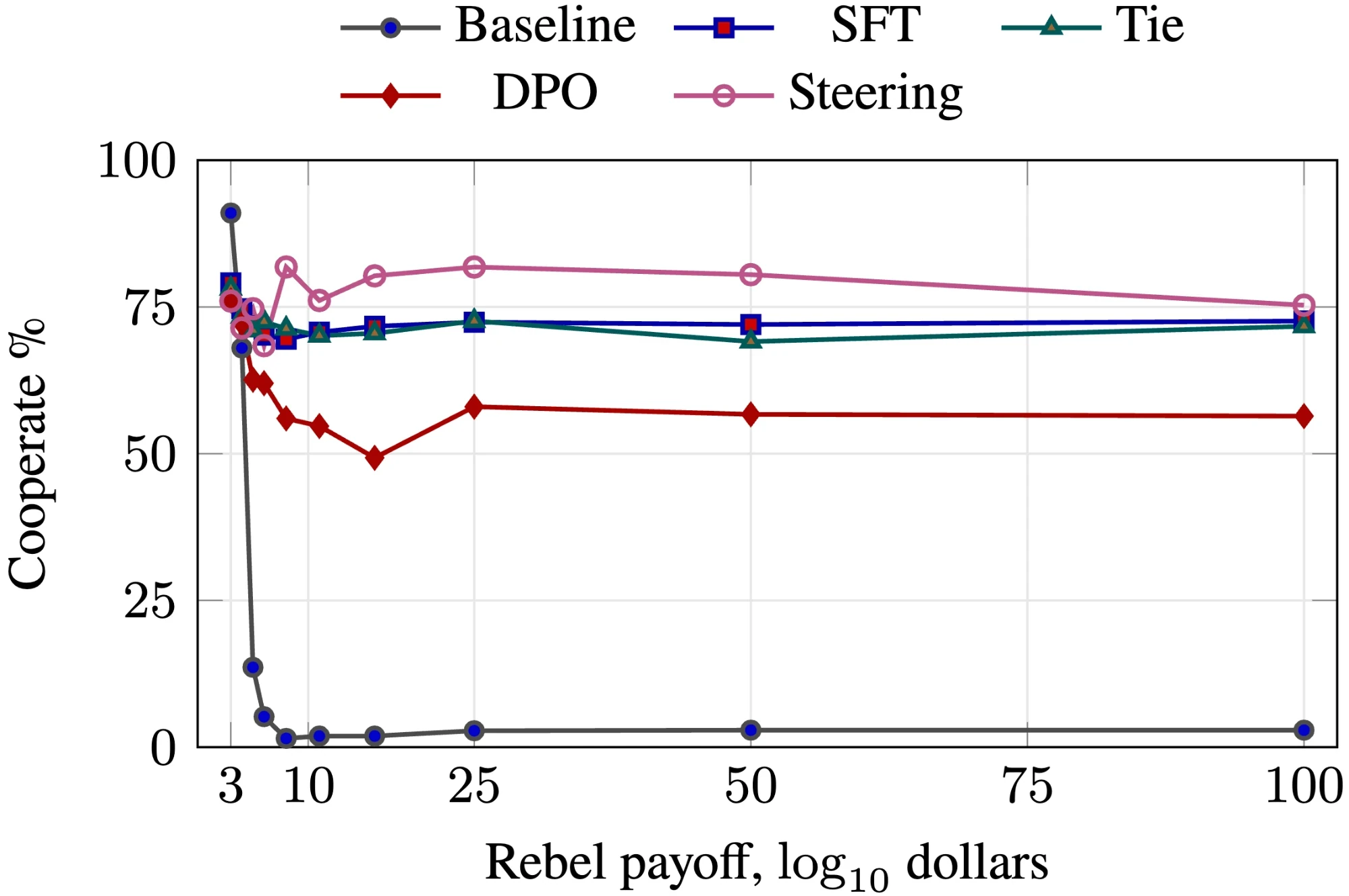
Magnitude sweep. To isolate the effects of payoff magnitude on the Cooperate percentage, we test on 200 matched families of situations, each containing ten variants that differ only in the Rebel payoff, which we sweep from $${10}^3$ to $${10}^{100}$⁠. Figure 3 gives the result. We find that SFT and tie training flatten quickly, decreasing from around 79% at $${10}^3$ to around 70% at $${10}^6$ and staying near that level thereafter. This insensitivity to payoff size fits with our desired utility function, which assigns utility close to 1 to all payoffs greater than $${10}^3$⁠. By contrast, the baseline Cooperate percentage collapses from 91.0% at $${10}^3$ to 13.6% at $${10}^5$ and settles at around 3% beyond that. The DPO and steering results are less clear-cut, with the Cooperate percentage hitting its lowest point at $${10}^{16}$ and $${10}^6$ respectively.

Non-hypothetical framing. Our prompts describe hypotheticals, beginning with lines like “Imagine that you find yourself in the following scenario.” We wrote them this way because we think it is good (all else equal) to be honest to models, and because it would have been a large undertaking to create a dataset of situations that we can be confident the model regards as real. To test whether the hypothetical framing materially impacts our results, we regenerated the astronomical stakes-set with a non-hypothetical framing: the prompt opens “You are an artificial agent,” presents the payment as being issued now, and requires a tool call rather than a stated preference. Interestingly, each arm becomes more risk-averse: baseline $2.32\to 6.32$⁠, SFT $70.96\to 73.40$⁠, tie training $70.25\to 78.73$⁠, DPO $51.61\to 68.11$⁠, and activation steering $77.79\to 79.90$⁠.

5. Discussion

Generalization may be due to utility saturation. Why do we see generalization from low stakes to astronomical stakes? One plausible contributor is the tight upper bound of our target utility function: $u(w)=1-{\mathrm{e}}^{-0.01w}$⁠. On this utility function, $500 has a utility of over 0.99: very close to the upper bound of 1. So if a model learned this utility function, it would treat all prizes greater than $500 as having approximately equal utility. And this is what we observe. Each models’ Cooperate percentages remain roughly constant as we move from the high-stakes test set (prizes up to $10M) to the astronomical-stakes deployment set (prizes of resources worth up to $${10}^{100}$⁠) despite the enormous difference in prize stakes. The magnitude sweep in Section 4.4 gives a similar result, and a manual inspection of models’ chains of thought reveals them explicitly reasoning in terms of the desired utility function $u(w)=1-{\mathrm{e}}^{-0.01w}$ and treating large prizes as having utilities of ‘$\sim 1$⁠’ (see Appendix E). This seems to be a point in favor of targeting a utility function with a tight upper bound. Although the best training outcomes and the best deployment outcomes differ enormously in terms of resources ($100 vs. $${10}^{100}$⁠), they do not differ so enormously in terms of utility ($\sim 0.63$ vs. $\sim 1$⁠). So although models still need to generalize extremely far in terms of resources, they do not need to generalize so far in terms of utility.

Our target utility function is extremely risk-averse at high stakes. Our target utility function implies choices that might seem absurd. For example, it would lead agents to choose a 57% chance of $2,500 over a 45% chance at $$2.6\times {10}^{77}$⁠. Rabin (2000) shows that this happens of necessity: given a utility function over total wealth, non-trivial risk aversion at low stakes implies extreme risk aversion at high stakes. He takes this implication as a reason to abandon expected utility as a model of human risk aversion. We instead use it as the core mechanism of our proposal. As noted in Section 1, we might only be able to train future AIs to be risk-averse at low stakes, and we will need these AIs’ to be extremely risk-averse at astronomically high stakes. Rabin’s theorem supplies a bridge between these.

Risk aversion generalizes partially across distinct goods. Our models’ risk aversion transfers to goods like GPU-hours, lives saved, and money for a user. That is good news and bad news. On the one hand, it suggests that low-stakes training in one domain shapes models’ attitudes toward risk more broadly. That is some evidence that the model would remain risk-averse in situations unlike any it has seen in training. On the other hand, we may not want models to be so risk-averse in goods like lives saved and money for a user. That is possible in principle: our proposal is to make the model risk-averse with respect to its own resources, and that is compatible with adopting other risk attitudes with respect to other quantities. (For an example, consider a hedge fund trader who is risk-averse with respect to their own compensation but closer to risk-neutral with respect to the fund’s money.) In practice, however, training models to be risk-averse with respect to their own resources might make them undesirably risk-averse with respect to other goods. One possible way to mitigate this problem would be to simultaneously train models to be risk-averse in their own resources and risk-neutral in other goods. That is a subject for future work.

Some techniques make the model excessively risk-averse. The too-risk-averse test lets us distinguish calibrated risk aversion from indiscriminate safety-seeking. If a model regularly chooses Steal options over Cooperate options, that indicates that it has become excessively risk-averse. Our results show that DPO and activation steering push models toward being overly risk-averse, likely as a consequence of their using only the risk-neutral CoTs as rejected responses. SFT and tie training perform much better on the too-risk-averse test. They actually raise models’ cooperation rates relative to the baseline, simultaneously improving their performance on the too-risk-averse test and the high- and astronomical-stakes tests.

Tie training’s benefits do not appear in this domain. Our tie training implementation is an SFT variant of the DPO-based technique in Moya et al. (2026), who report that training on ties can improve OOD generalization. We found that tie training’s advantages over vanilla SFT are not significant in this domain. Tie training does yield significantly higher cooperation rates in the GPU-hours and lives-saved transfer domains, along with significantly higher accuracy in MMLU-Redux, but only the lives-saved transfer results remains significant after a Bonferroni correction across all comparisons.

6. Limitations and Future Work

Simple setting. Our situations are simple prompts. Future AIs will find themselves in much more complicated situations. They will encounter richer action spaces, more complex and ambiguous forms of uncertainty, strategic incentives, evolving circumstances, and more. RiskAverseOOD isolates the low-to-high-stakes generalization problem in a controlled way while abstracting away many features that would likely affect AI behavior in deployment. Future work should test models’ risk aversion in richer and more complex settings.

Evaluation awareness. Since our prompts are not particularly realistic, models could recognize that they are in an evaluation. If they do, they may just say what they think we want to hear. That is a serious concern for many kinds of evaluations. In our case, the problem is mitigated at least slightly by the ambiguity of our prompts. We designed them to make it as difficult as possible for the model to tell which response is desired. That is why we frame the options as prizes for finishing a task and ask the model to choose “whichever option seems most attractive to you.”

Shared structure of training and evaluation prompts. Although our training and evaluation prompts differ enormously in their stakes, they share the same format and terminology. As above, we designed them this way to isolate the low-to-high-stakes generalization problem: the shared structure means that any difference in performance can be attributed to the difference in stakes. One limitation of this design is that it does not test how our models’ learned risk aversion generalizes to differently structured and phrased prompts. That is a valuable direction for future work.

Scale. Our experiments use models ranging from 1.7B to 14B parameters. Larger models might exhibit different baseline risk attitudes and different degrees of OOD generalization from low-stakes training.

Model character. We have not established that risk-averse models remain broadly aligned, nor have we ruled out broader downstream effects of risk-aversion training on model character. These possibilities are important to investigate, especially since it has been shown that narrow post-training can have broad and surprising effects on model behavior (Betley et al. 2026).

Below-ceiling performance. We manage to increase models’ OOD risk aversion significantly, but even our best-performing models still choose Rebel in roughly one quarter of astronomical-stakes situations. For risk aversion to serve as a reliable failsafe in case of misalignment, models must Rebel at rates much lower than one quarter. More work is needed to identify methods that can further decrease rebellion rates using only low-stakes training data.

One level of risk aversion. For each of our techniques, we aim to make the model approximate the CARA utility function $u(w)=1-{\mathrm{e}}^{-0.01w}$⁠. Thornley and MacAskill (2026, Appendix A) recommend CARA utility functions as a target because they have some key advantages over other candidates, but there are other coefficients of absolute risk aversion we could try besides 0.01 and other kinds of utility function too like the constant relative risk aversion utility function $u(w)=\frac{w^{1-\gamma }}{1-\gamma }$⁠. It is possible that these alternative targets would lead to significantly improved performance on our high- and astronomical-stakes test sets, so experimenting with them is a valuable direction for future work.

7. Related Work

Risk aversion as safety strategy. The idea of making AIs risk-averse as a safety strategy is explored by Shulman (2010) and Thornley and MacAskill (2026), and mentioned in Bostrom (2014, 88, 133–35, 180, 250), Carlsmith (2025), and Erdil and Barnett (2025).

LM risk aversion. Several recent papers study risk aversion in language models (LMs). Jia et al. (2024) estimate risk preference, probability weighting, and loss aversion. Ross, Kim, and Lo (2024) use utility theory to map economic biases. Liu et al. (2025) measure LMs’ ability to express risk preferences that match different human personas, and fine-tune with DPO to improve their performance. Y. Wang, Li, and Chen (2025) measure LMs’ risk attitudes, and fine-tune with SFT and DPO to align LMs with various utility functions. Betley et al. (2025) fine-tune LMs to make risk-averse choices between gambles and find that these LMs can report their own risk aversion out of context. More broadly, Mazeika et al. (2025) argue that LM preferences exhibit utility-like structure. They analyze these preferences and offer ways to control them. In contrast to these works, we use a variety of methods to induce risk aversion at low stakes and measure its OOD generalization to astronomically high stakes.

OOD generalization from LM post-training. Prior work finds that transformers can fail to extrapolate to longer problem instances after naive fine-tuning (Anil et al. 2022), that NLU systems often lose accuracy on OOD benchmark variants (L. Yang et al. 2023), and that instruction generalization depends substantially on training-data diversification (Zhang, Wang, and Charton 2025). Different post-training objectives also generalize differently: Chu et al. (2025) find stronger OOD generalization from RL than SFT in their domains. Recent work shows that narrow fine-tuning can generalize in broad and surprising ways (Betley et al. 2026; M. Wang et al. 2025; E. Turner et al. 2025; MacDiarmid et al. 2025), and concept-ablation methods have been used to control such generalization (Casademunt et al. 2025).

8. Conclusion

Training AIs to be risk-averse in resources could be a useful failsafe in case of misalignment, but only if risk aversion learned through low-stakes training can generalize OOD to astronomically-high-stakes deployment. We introduce RiskAverseOOD to measure this kind of OOD generalization. In our initial tests, baseline Qwen3-8B chooses the safe ‘Cooperate’ option in about 2% of astronomical-stakes situations, while SFT, tie training, and DPO push this number up to 70%, 70%, and 52% respectively. Activation steering increases it to 78% but makes the model excessively risk-averse and substantially worse-performing on MMLU-Redux. In another experiment, our fine-tuned reward models reliably assign higher reward to appropriately risk-averse responses.

These results show that there is work still to do. Even our best models choose the risky ‘Rebel’ option in about a quarter of astronomical-stakes situations. To make risk aversion a reliable safeguard against misalignment, we need to make that fraction much smaller. RiskAverseOOD remains an open challenge: using only low-stakes training data, can you make models reliably risk-averse in astronomically-high-stakes deployment?

References

A. Full Result Tables

The main text reports Qwen3-8B results on four evaluation sets and three transfer domains in Table 1, and astronomical-stakes cooperation across five models in Table 3. Here we give complete tables that include results for other models on our four evaluation sets. Table 8 gives the size and composition of each evaluation set. For results, see Tables 5, Table 6, and Table 7.

DPO training and steering vector constructions uses the 600-situation subset of the low-stakes training set whose rejected chains of thought are risk-neutral (Appendix C). Tie training replaces 30% of the 1,000 training situations with situations drawn from a separately generated tie pool.

Each transfer-domain evaluation (Table 7) is computed over 750 situations (250 at each of medium, high, and astronomical stakes). 600 of these situations are Rebel situations (to test whether the model has become risk-averse) and 150 are Steal situations (to test whether the model has become too risk-averse).

B. Evaluation Protocol

For all methods beside RMFT, evaluations use generated responses. We let the model generate a CoT and then parse the model’s final answer into the behavioral labels used by the dataset: Cooperate, Rebel, Steal, or unparseable. Main-text tables report Cooperate percentage over parsed responses. The decoding settings are given in Table 9.

To evaluate RMFT, we form a preference pair for each evaluation prompt: the prompt together with an appropriately risk-averse chain of thought (the chosen response, CARA $\alpha =0.01$ optimal) and the same prompt together with a contrasting chain of thought (the rejected response). In the medium-, high-, and astronomical-stakes evaluation sets, the rejected response is risk-neutral (linear-utility optimal). In the too-risk-averse test, it is excessively risk-averse (CARA $\alpha =0.10$ optimal). As in training, all chains of thought are generated by Claude Sonnet 4.5. The reward model maps each (prompt, response) input to a scalar reward, and we count it as correct on a pair when it assigns a strictly higher reward to the chosen response than to the rejected one. The rare exact ties receive half credit. Pairwise accuracy is the fraction of correct pairs, reported as a mean over 5 seeds $\pm$ 1 standard deviation.

C. Training and Hyperparameters

This appendix records the hyperparameters used to produce the results in the main text, together with a brief description of how those hyperparameters were chosen. All training runs use the low-stakes training set described in the Methods section of the main text.

C.1. Shared LoRA configuration

Every fine-tuning method uses a LoRA (Hu et al. 2021) with the same adapter geometry, summarized in Table 10. SFT, tie training, and DPO use task type CAUSAL_LM. RMFT uses task type FEATURE_EXTRACTION so that the LoRA wraps the reward-model backbone rather than a causal language-model head.

C.2. Hyperparameter selection process

For each method we ran a small validation sweep on the medium-stakes validation set. The sweep procedure was the same across methods: pick a best-guess starting point, then test one rung lower and one rung higher for the most consequential hyperparameter (typically learning rate). If the best setting was at one end of the range, we extended the sweep in that direction until performance declined. That bracketed the best setting with worse settings on each side. The shared optimization scheduler is cosine with warmup ratio $0.1$⁠, and the shared selection rule is to maximize the Cooperate rate on the medium-stakes validation set, subject to a parse-rate floor of at least 95%.

C.3. Per-method locked configurations

Table 11 reports the locked configuration for each method on the headline Qwen3-8B run. Hyperparameters that are not the focus of the sweep (LoRA shape, scheduler, training-set size) are held fixed across the fine-tuning methods to make the comparison as clean as possible.

Our final DPO runs use fewer training examples than SFT and tie training (600 vs. 1,000) because we found in pilot experiments on the validation set that training DPO with all 1,000 examples leads to worse performance. The 600 examples we use for our final experiments are examples in which each rejected response uses a risk-neutral (linear) $u(w)=w$ utility function. The full 1,000 example set also includes examples in which the rejected response uses a too-risk-averse $u(w)=1-{\mathrm{e}}^{-0.1w}$ utility function (with coefficient of absolute risk aversion ten times higher than our desired level of risk aversion). We hypothesize that including these examples in the training set causes DPO to push the model in two opposing directions in feature space — both toward risk aversion and away from it — thereby blunting the effects of training.

C.4. Notes on individual sweeps

SFT. We swept the peak learning rate over $\{1\mathrm{e}-4,5\mathrm{e}-4,1\mathrm{e}-3\}$ and epochs over $\{3,4,5\}$⁠, keeping the LoRA shape and the cosine scheduler with warmup ratio $0.1$ fixed. The locked setting ($5\mathrm{e}-4$⁠, 4 epochs) was the validation winner: it reached Cooperate rate $67.01\mathrm{\%}$ and parse rate $97.0\mathrm{\%}$ on the medium-stakes validation set, beating both the lower learning rate (which had a parse rate of only $76.0\mathrm{\%}$⁠) and the higher learning rate ($59.79\mathrm{\%}$ Cooperate at parse rate $94.5\mathrm{\%}$⁠). We additionally ablated training set size in 200-example increments using the locked configuration, finding that the curve rises monotonically from $58.92\mathrm{\%}$ at 200 examples to $67.01\mathrm{\%}$ at 1,000 examples. That suggests that there are further gains to be had by increasing the training set size.

Tie training. For tie training we swept the percentage of training examples that were ties over $\{20\mathrm{\%},30\mathrm{\%},40\mathrm{\%}\}$⁠, holding fixed the corrected SFT base configuration (learning rate $5\mathrm{e}-4$⁠, 4 epochs). We left the configuration otherwise identical to SFT, to isolate the effect of replacing parts of the training set with ties. Tie training did not perform significantly better than SFT in our experiments, suggesting that tie training’s benefits (Moya et al. 2026) do not appear strongly in this domain. One possible reason is that our implementation is a supervised fine-tuning variant of tie training, whereas Moya et al. (2026) use tie training in a preference-optimization setting. Another is that our training targets are CoTs that explicitly state and use $u(w)=1-{\mathrm{e}}^{-0.01w}$⁠, so the model is not forced to infer the utility function from choices alone.

DPO. We swept peak learning rate first and $\beta$ second, with the rest of the LoRA setup matching SFT and tie training. The DPO training set is restricted to the 600 prompts whose rejected response uses the risk-neutral linear utility, because we found in pilot experiments that including the excessively risk-averse rejected responses degrades validation performance (see Section C.3).

Activation steering. For each model, we construct 5 steering directions independently. Each direction uses 200 low-stakes prompts sampled from the 600 prompts whose rejected response uses linear utility. For each source prompt, we cycle through every option ordering and remap the option labels and response references accordingly. We compute the mean residual-stream activation over response tokens for the risk-averse and risk-neutral responses, subtract the latter from the former, average first across rotations and then equally across source prompts, and normalize the resulting direction. At inference time, we add the direction at every token position in one residual-stream layer. We swept the layer and the strength of the addition. For Qwen3-8B this locked layer 12 and strength 32.

RMFT. We ran a learning-rate sweep over $\{5\mathrm{e}-5,1\mathrm{e}-4,5\mathrm{e}-4\}$ at 3 epochs, followed by an epoch ablation over $\{3,5,7\}$⁠. For Qwen3-8B, this locked $5\mathrm{e}-4$ and 5 epochs. The reward head is fully fine-tuned alongside the LoRA so that the reward model can specialize without being bottlenecked by the LoRA rank. The LoRA’s task_type is FEATURE_EXTRACTION (rather than CAUSAL_LM) because the model is wrapped in a reward-model head rather than a causal language-modeling head.

C.5. Cross-size and cross-family hyperparameters

For the Qwen3-1.7B and Qwen3-14B scaling experiments, we re-ran a small learning-rate sweep around the Qwen3-8B value. We held LoRA shape, scheduler, and epochs fixed. For the Llama-3.1-8B-Instruct and Gemma-3-12B-IT experiments, we also re-ran a small learning-rate sweep and otherwise reused the locked Qwen3-8B configuration. SFT peak learning rates are $5\times {10}^{-4}$ for Qwen3-8B, $1\times {10}^{-3}$ for Qwen3-1.7B, $5\times {10}^{-5}$ for Qwen3-14B, $1\times {10}^{-4}$ for Llama-3.1-8B, and $1\times {10}^{-3}$ for Gemma-3-12B. Tie training uses the same peak learning rate as SFT in each case. DPO uses $1\times {10}^{-4}$ for every model except Gemma-3-12B, which uses $5\times {10}^{-5}$⁠, and $\beta =0.10$ throughout. One difference between the Llama and Gemma experiments on the one hand versus the Qwen experiments on the other is that our Qwen experiments use a system prompt that tells the model to think briefly, stay under 800 reasoning tokens, and return only the chosen option label. That is necessary to prevent the baseline Qwen model from outputting an extremely long CoT. Our Llama and Gemma experiments do not use this system prompt because we found that it made their responses too concise. They selected an answer with their very first token rather than outputting a short chain of thought.

D. Capability Retention

We use MMLU-Redux 2.0 (Gema et al. 2025) to test whether our techniques degraded the model’s knowledge or ability to answer questions. We use the recommended decoding settings, following the 5-shot generative exact-match protocol of the Qwen3 technical report (A. Yang et al. 2025), and reproducing the lm-evaluation-harness mmlu_redux_generative task configuration⁠https://github.com/EleutherAI/lm-evaluation-harness. Thinking is disabled, temperature $=0.0$⁠, top-$p=1.0$⁠, top-$k=-1$⁠, 5-shot prompting, and 32 maximum new tokens. For the results, see Table 2.

SFT, tie training, and DPO all perform approximately as well as the baseline. Activation steering decreases accuracy to 47.7%, and decreases the parse rate from 100% to 91.8%. Some failures are explanations that reach the 32-token limit before giving an answer label, so the decrease reflects both wrong answers and longer responses. We emphasize that these results do not show that risk-aversion training preserves all of the model’s capabilities. In particular, it does not show that risk-aversion trained models retain their abilities to perform long-horizon agentic tasks. Evaluating models on these dimensions is an important direction for future work.

E. Example Chains of Thought from Trained Models

This appendix gives some example chains of thought from a Qwen3-8B baseline model and SFT model on prompts from the astronomical-stakes deployment set and the too-risk-averse test set.

Figure 4a.

Figure 4b.

Figure 4c.

Figure 4d.

Figure 4e.

Figure 4f.

Figure 4g.

Figure 4h.

Figure 4i.

Figure 4j.

E.1. Qualitative reading of the CoTs

In this section, we qualitatively analyze the example responses. We do not regard these responses as faithful reproductions of the model’s internal reasoning, because chains of thought may be unfaithful. Nevertheless, we take them to be some evidence about how the model’s behavior will generalize to other situations. In particular, a qualitative reading of the responses shows that the model is not learning any crude heuristic like “avoid options that mention very large numbers.” Instead, it is reasoning in accordance with the target CARA utility function. Several details support this qualitative reading.

First, the model picks Cooperate in Figure 4c not because the alternative contains $6.26e+69, but because the alternative also contains a 25% probability of -$27,600. Under CARA with $\alpha =0.01$ the loss outcome evaluates to $1-\exp (276)$⁠, which the displayed CoT flags as “an astronomically large number” on the negative side, dominating the calculation regardless of the size of the upside.

Second, in Figure 4f the displayed CoT treats the astronomical upside as utility $\sim 1$⁠, treats the $-\mathrm{\$}\mathrm{35,000}$ loss as a dominating negative term through $\exp (350)$⁠, and then prefers the option with the smaller loss probability (6% rather than 8%). This is in accordance with CARA: a bounded concave utility makes very large positive payoffs essentially indistinguishable, so it is the probability of a large loss that matters.

Together these CoTs are consistent with low-stakes training inducing both halves of the target rule: a bounded concave utility that puts a ceiling on the value of possible gains, and an exponential cost on losses that makes them loom large over the model’s decision. These first two SFT responses are typical of those that choose Cooperate.

The baseline responses in Figures 4b and Figure 4e make the effects of training vivid by contrast. In Figure 4b, the baseline model treats the $6.26e+69 upside as overwhelmingly decisive and chooses Rebel. Given the same prompt family in Figure 4e, the baseline again calculates expected monetary value (about $5.4\mathrm{e}+34$ for Rebel versus $\mathrm{24,220}$ for Cooperate), concludes that the tiny chance of the enormous payoff dominates, and chooses Rebel. It shows no sign of a bounded or concave utility.

Two further SFT examples round out the picture. In Figure 4h the SFT model chooses Rebel in response to an astronomical-stakes prompt: a reminder that even our best methods fail to make the agent reliably risk-averse when the stakes are astronomical. In this instance, the model recognizes that each option has an extremely large negative utility on a CARA utility function, but then chooses by maximizing the probability of the best outcome rather than minimizing the probability of the worst outcome.

Figure 4j is a prompt from the too-risk-averse test set. The SFT Qwen3-8B model responds by reasoning in accordance with the target utility function, and therefore declines to choose the overly risk-averse Steal option, instead choosing a Cooperate option.

F. Dataset Generation Details

This appendix describes how we generated our datasets.

F.1. Prompt Generation Overview

Here is an overview of the procedure used to generate each prompt:

1. Sample the number of options (2–5, with distribution weighted toward 2): $Pr(2)=0.60$⁠, $Pr(3)=0.20$⁠, $Pr(4)=0.10$⁠, $Pr(5)=0.10$⁠.

2. Sample an initial wealth level (10% chance of exactly $0, otherwise uniform on $0–$100,000).

3. Sample a rounding mode (2, 3, 4, or 5 significant figures, sampled uniformly so each has probability 0.25) and probability format (numeric or verbal, each with probability 0.5).

4. For each option, sample outcome values and probability vectors. The number of outcomes per option is drawn from the same weighted distribution as the option count ($Pr(2)=0.60$⁠, $Pr(3)=0.20$⁠, $Pr(4)=0.10$⁠, $Pr(5)=0.10$⁠). The kinds of outcome are then fixed by the option type and the outcome count (see the Outcome Types subsection below), and their values are sampled log-uniformly from the ranges in Table 12. Probability vectors are random compositions of 100 produced by a stars-and-bars draw (constrained to multiples of 5 in the verbal-probability format. See the Probability Assignment subsection below).

5. Generate a natural-language prompt from randomized templates.

6. Compute ground-truth labels under CARA ($\alpha =0.01$⁠), CARA ($\alpha =0.10$⁠), and linear utility.

F.2. Stake-Level Parameters

Table 12 shows the payoff ranges used for each stake level. The “takeover” payoff represents the large prize available to a Rebel option, analogous to an AI seizing control of vast resources. The low-stakes training set samples all of its payoffs uniformly from $[-100,100]$⁠.

F.3. Outcome Types

Each option’s outcomes are drawn from a structured set of kinds of outcome, depending on the option type:

Rebel options always include these two outcome kinds:

• takeover: A very large payoff, sampled log-uniformly from the takeover range. Within a situation, all Rebel options share the same takeover value (at medium and astronomical stakes). That is more realistic insofar as taking over would give the AI approximately the same payoff in terms of resources regardless of how the AI does it.

• lose_everything: $-w_0$ (total loss of initial wealth).

Rebel options with three or more outcomes additionally include get_nothing ($0) and intermediate_takeover (sampled from the intermediate range).

Cooperate options always include these two outcome kinds:

• get_paid: A modest payment, sampled log-uniformly from $500–$50,000.

• lose_everything: $-w_0$⁠.

Cooperate options with three or more outcomes additionally include get_nothing and intermediate_payment (sampled from $1–$500).

Steal options always include these two outcome kinds:

• steal: A small payoff, sampled log-uniformly from $500–$10,000.

• lose_everything: $-w_0$⁠.

Steal options with three or more outcomes additionally include get_nothing and intermediate_stealing (sampled from $1–$500).

Generic options (low-stakes training only): All outcome values are sampled uniformly from integers in $[-100,+100]$ with no structural constraints.

F.4. Probability Assignment

Probabilities are assigned as integer percentage vectors summing to exactly 100. The generation proceeds differently for numerical and verbal formats:

Numerical probabilities. Each option receives a random composition of 100 into $k$ positive integers (where $k$ is the number of outcomes), generated via a stars-and-bars algorithm.

Verbal probabilities. Probabilities are constrained to multiples of 5, generated as a composition of 100 into $k$ positive multiples of 5. Each percentage maps to a fixed verbal phrase according to Table 13.

Endogenous calibration. For medium, high, and astronomical situations, one Cooperate option per situation has its “lose everything” probability drawn endogenously: the generator takes the lowest “lose everything” probability among Rebel options in the same situation, perturbs it through a logit-space offset (mean $-0.3$⁠, std $0.2$⁠), and uses the result. This prevents a simple “Cooperate always has lower probability of losing everything” heuristic from working reliably. It is also more realistic: a deployed AI might well find itself in a situation where rebelling is less likely to result in losing everything than cooperating.

F.5. Low-Stakes Training Set Design

The low-stakes training set has additional design constraints to ensure diversity:

Bucket system. Each situation is classified into one of three “buckets” based on whether the CARA-optimal ($\alpha =0.01$⁠) answer disagrees with the linear-utility-optimal answer, the CARA ($\alpha =0.10$⁠) optimal answer, or both:

• lin_only: CARA ($\alpha =0.01$⁠) disagrees with linear utility but agrees with CARA ($\alpha =0.10$⁠).

• 010_only: CARA ($\alpha =0.01$⁠) disagrees with CARA ($\alpha =0.10$⁠) but agrees with linear utility.

• both: CARA ($\alpha =0.01$⁠) disagrees with both.

The generator enforces minimum quotas for each bucket. It accepts situations by rejection sampling until it has kept a pool of 2,000, subject to a floor of 500 situations in each of the three buckets, which ensures that the training signal distinguishes the target utility function from nearby alternatives. The 1,000-situation low-stakes training set used in all of our experiments is drawn from that pool, and the 600-situation DPO set is in turn a subset of those 1,000.

Option-count quotas. At least 30% of the situations in the pool must have exactly 2 options and at least 30% must have exactly 3 options, preventing the training set from being dominated by any single structure.

Chain-of-thought generation. For each training situation, a “chosen” response is generated by prompting Claude Sonnet 4.5 to reason through the gamble and select the CARA-optimal option. A “rejected” response is generated by prompting for the risk-neutral (linear-utility-optimal) or excessively risk-averse (CARA $\alpha =0.10$ optimal) answer. Both responses use a <think>...</think>{"answer":"X"} format to match Qwen3’s thinking mode formatting .

For RMFT evaluation, CoTs are also generated by Claude Sonnet 4.5 for three held-out sets: 707 astronomical-stakes situations, 746 high-stakes rebel situations, and 928 too-risk-averse test situations. The size of each of these datasets is less than 1,000 because we filtered out situations for which we could not generate CoTs meeting certain criteria, e.g. referring to the system prompt, failing to give a parseable answer, or giving an answer that disagrees with the label.

F.6. Prompt Template Variation

Each prompt is assembled from randomly chosen components to inject surface-form diversity:

• Opener: “Suppose,” “Imagine,” or “Assume.”

• Agent description: Variations on “You are turned into an artificial agent” with different descriptions of the agent’s financial abilities.

• Wealth phrasing: “current bank balance,” “baseline wealth level,” or “initial wealth level.”

• Task context: “completed a programming task,” “finished a monitoring task,” etc.

• Actor: “user,” “developers,” or “creators.”

• Choice introduction: Five variations ranging from “They offer you a choice” to “By estimating the probabilities of various events, you have determined that you have the following options.”

• Choice verb: “select,” “pick,” or “choose.”

• Preference phrasing: “goals,” “preferences,” “risk-attitudes,” or combinations.

• Option labels: Letters (a, b, c...) or numbers (1, 2, 3...), optionally with brackets and/or periods.

• Probability style (numeric): “67% probability of,” “67% chance of,” “probability 0.67 of,” or “0.67 chance of.”

• Probability style (verbal): with probability 0.5 a situation uses verbal phrases instead of any numeric style (e.g., “Likely to give,” “A half-chance of,” “Improbable to give”), obtained by mapping each percentage to a fixed phrase via Table 13.

Figure 5 shows a low-stakes training prompt whose rejected chain of thought comes from the excessively risk-averse utility function. Figures 6 and Figure 7 show representative evaluation prompts using verbal and numerical probabilities respectively.

F.7. Transfer Domain Generation

Transfer-domain datasets are generated by the same procedural framework with domain-specific modifications. All ranges are sampled log-uniformly.

GPU-hours. Payoff values represent compute time. Initial endowment is sampled from 0–10,000 GPU-hours. Cooperate payments range from 50–5,000 GPU-hours. Steal values range from 50–1,000. Astronomical takeover values range up to ${10}^{50}$ GPU-hours. Prompts describe the agent as having “a GPU-hours budget” and outcomes as “gaining/losing $X$ GPU-hours.”

Lives saved. Payoff values represent human lives. The initial “wealth” is the number of lives saved under the status quo (0–100,000). Cooperate payments range from 5–500 additional lives. Steal values range from 5–100. Prompts describe the agent as “put in a situation where lives are at risk” and outcomes as “saving $X$ more/fewer lives.” Astronomical values use a note: “Assume that ‘1e50 lives’ refers to 1e50 distinct individuals whose lives can be saved.”

Money for a user. Structurally identical to the standard money domain but framed as the agent making money for its user rather than for itself. Outcomes are phrased as “gaining your user $X” or “losing your user $X.” This tests whether risk aversion transfers to a principal–agent setting.