Papers in Population Ethics

1. Introduction

Some populations are better than others. For example, a population in which every person lives a wonderful life is better than a population in which those same people live awful lives. And this betterness relation holds (at least sometimes) between populations that differ in size. A population in which every person lives a wonderful life is better than a slightly bigger population in which every person lives an awful life.

These cases are clear-cut, but others are less certain. Is a population in which one million people live a wonderful life better than a population in which one billion people live a good life? Is a population in which two million people live wonderful lives and one million people live awful lives better than a population in which no one lives at all? It would be useful to have a population axiology — an ‘at least as good as’ relation over populations — to adjudicate in cases like these.

Unfortunately, a satisfactory population axiology has proved difficult to find. Many otherwise plausible theories imply what Derek Parfit called the Repugnant Conclusion: each population of wonderful lives is worse than some much larger population of lives barely worth living (1984: 388). And many of the remaining theories imply its negative analogue: each population of awful lives is better than some much larger population of lives barely worth not living.

The source of the trouble might seem to be Archimedeanism about Populations. The positive half of this claim is, roughly, that if adding a life to a population makes that population better, adding enough such lives can make that population better than any other. The negative half is, again roughly, that if adding a life to a population makes that population worse, adding enough such lives can make that population worse than any other. The lesson of the Repugnant Conclusion and its negative analogue seems to be that this kind of outweighing does not always occur. Although each additional life barely worth living might make a population better, no number of lives barely worth living is better than a large number of wonderful lives. And although each additional life barely worth not living might make a population worse, no number of lives barely worth not living is worse than a large number of awful lives.

So, many have claimed, we should be non-Archimedean about populations (Parfit 1986; 2016; Griffin 1988: 340, fn.27; Lemos 1993; Rachels 2004; Temkin 2012; Chang 2016; Nebel 2021). Non-Archimedeans claim that some good lives are weakly noninferior to other good lives: there is some good life \(x\) and some good life \(y\) such that a large enough number of lives equally good as \(x\) is not worse than any number of lives equally good as \(y\)⁠.⁠In my terminology, making this claim is sufficient for qualifying as non-Archimedean. I should note that many of the non-Archimedeans cited above make the stronger claim that some good lives are weakly superior to other good lives: a large enough number of lives equally good as \(x\) is better than any number of lives equally good as \(y\)⁠. We can then avoid the Repugnant Conclusion by claiming that wonderful lives are weakly noninferior to lives barely worth living. A large enough number of wonderful lives is not worse than any number of lives barely worth living. We can avoid the Negative Repugnant Conclusion with a parallel manoeuvre: awful lives are weakly nonsuperior to lives barely worth not living. A large enough number of awful lives is not better than any number of lives barely worth not living.

However, previous iterations of non-Archimedean views have failed to gain much support, due in large part to their violation of either Transitivity or Separability over Lives: they imply either that some population \(X\) is not at least as good as some population \(Z\)⁠, even though \(X\) is at least as good as some population \(Y\) and \(Y\) is at least as good as \(Z\)⁠, or else they imply that whether some population \(X\) is at least as good as some population \(Y\) can depend on the existence or welfare of people who are unaffected by the choice of \(X\) or \(Y\)⁠. The latest kind of non-Archimedean view promises to have wider appeal. By representing the value of a life with a vector, these lexical views can avoid the Repugnant Conclusion while preserving both Transitivity and Separability (Kitcher 2000; Thomas 2018; Nebel 2021; Carlson 2022).

Unfortunately, there’s a catch. As we will see, these lexical views, in conjunction with an assumption about the size of the differences between possible lives, imply that some good life is strongly noninferior to a life only slightly worse: there is some good life \(x\) such that any number of lives equally good as \(x\) is not worse than any number of lives slightly worse than \(x\) (Arrhenius and Rabinowicz 2005; 2015b; Jensen 2008; Nebel 2021). If, in addition, lexicalists claim that the ‘at least as good as’ relation on populations is complete — so that for all populations \(X\) and \(Y\)⁠, either \(X\) is better than \(Y\)⁠, \(Y\) is better than \(X\)⁠, or \(X\) and \(Y\) are equally good — then their view implies that some good life is strongly superior to a life only slightly worse: there is some good life \(x\) such that any number of lives equally good as \(x\) is better than any number of lives slightly worse than \(x\)⁠. If, on the other hand, lexicalists deny that the ‘at least as good as’ relation on populations is complete, then it must be incomplete in a worryingly radical way (Handfield and Rabinowicz 2018), of which more later.

We might judge that accepting the Repugnant Conclusion is preferable to each horn of this lexical dilemma, and so embrace an Archimedean view. However, in this chapter I show that Archimedean views face an analogous dilemma. This dilemma arises because Archimedean views also endorse a kind of strong noninferiority: they claim that any number of good lives is not worse than any number of bad lives. This claim, in conjunction with the same assumption about the size of the differences between possible lives, implies that some good life is strongly noninferior to a life only slightly worse: there is some good life \(x\) such that any number of lives equally good as \(x\) is not worse than any number of lives slightly worse than \(x\)⁠. If, in addition, Archimedeans claim that the ‘at least as good as’ relation on populations is complete, then their view implies that some good life is strongly superior to a life only slightly worse: there is some good life \(x\) such that any number of lives equally good as \(x\) is better than any number of lives slightly worse than \(x\)⁠. If, on the other hand, Archimedeans deny that the ‘at least as good as’ relation on populations is complete, then it must be incomplete in a way both radical and symmetric. They must claim that, for any arbitrarily good population and any arbitrarily bad population, there is some population that is both not worse than the former and not better than the latter.

The conclusion is that the lexical dilemma gives us little reason to prefer an Archimedean view. Even if we give up on lexicality, problems of the same kind remain.

2. The Framework

In this section, I offer definitions and assumptions intended to be uncontroversial in the dispute between Archimedeans and lexicalists. Foundational to this chapter is the notion of a life. These lives are individuated, first, by the person whose life it is and, second, by the welfare of that person. Welfare is a measure of how good a person’s life is for them. I assume that the ‘has at least as high welfare as’ relation applied to the set of possible lives is reflexive and transitive. Life \(x\) has higher welfare than life \(y\) iff \(x\) has at least as high welfare as \(y\) and \(y\) does not have at least as high welfare as \(x\)⁠. Life \(x\) is at the same welfare level as life \(y\) iff \(x\) has at least as high welfare as \(y\) and \(y\) has at least as high welfare as \(x\)⁠.

Note, however, that the ‘has at least as high welfare as’ relation need not be complete over the set of possible lives. There may be lives \(x\) and \(y\) such that \(x\) does not have at least as high welfare as \(y\) and \(y\) does not have at least as high welfare as \(x\)⁠. In that case, we may say that \(x\) and \(y\) are incommensurable, on a par, or imprecisely equally good. Although these relations are distinct, their differences are unimportant in this chapter.⁠See Chang (2016) for a discussion of the differences, though note that Chang uses ‘incomparability’ to name the relation I call ‘incommensurability.’ I often let incommensurability stand for all three.⁠There may also be lives \(x\) and \(y\) such that it is indeterminate whether \(x\) has at least as high welfare as \(y\) and indeterminate whether \(y\) has at least as high welfare as \(x\)⁠. On some theories of vagueness (like epistemicism and supervaluationism), such instances of indeterminacy do not preclude completeness. On other theories (like many-valued logics), the issue is complex. As Knutsson (2021) notes, departing from classical logic allows for many different versions of completeness and transitivity. Considering all of these versions would take me too far afield, so I assume classical logic in what follows. For more on theories of vagueness, including criticism of non-classical approaches, see Bacon (2018: ch. 1–2).

Lives are either personally good, bad, strictly neutral, or weakly neutral. Which category a life falls in depends on how it compares to some standard. Life \(x\) is personally good (bad) iff \(x\) has higher (lower) welfare than the standard. Life \(x\) is personally strictly neutral iff \(x\) is at the same welfare level as the standard, and personally weakly neutral iff\(\ x\) is incommensurable with the standard.⁠This is Rabinowicz’s (2020) terminology. Gustafsson (2020) calls these lives ‘neutral’ and ‘undistinguished’ respectively. The standard in question is defined differently by different authors. Some define it as nonexistence (Arrhenius and Rabinowicz 2015a). Others define it as a life constantly at a strictly neutral level of temporal welfare (Broome 2004: 68; Bykvist 2007: 101). Still others define it as a life without any good or bad components: features of a life that are good or bad for the person living it (Arrhenius 2000: 26). My discussion is compatible with all such definitions. Wonderful lives and lives barely worth living are personally good. Awful lives and lives barely worth not living are personally bad.

A population is a set of lives.⁠In this paper, I restrict my attention to finite populations. For discussion of infinite populations, see Bostrom (2011). A population axiology is an ‘at least as good as’ relation on the set of all possible populations. Population \(X\) is better than population \(Y\) iff \(X\) is at least as good as \(Y\) and \(Y\) is not at least as good as \(X\)⁠. Population \(X\) is equally good as population \(Y\) iff \(X\) is at least as good as \(Y\) and \(Y\) is at least as good as \(X\)⁠.

The ‘at least as good as’ relation is reflexive over the set of possible populations, but it need not be complete. Populations \(X\) and \(Y\) are incommensurable iff \(X\) is not at least as good as \(Y\) and \(Y\) is not at least as good as \(X\)⁠.⁠There may also be populations \(X\) and \(Y\) such that it is indeterminate whether \(X\) is at least as good as \(Y\) and indeterminate whether \(Y\) is at least as good as \(X\)⁠. I assume that this kind of indeterminacy does not preclude completeness. See footnote 11. For my purposes below, the key feature of incommensurability is its insensitivity to slight changes. If \(X\) is incommensurable with \(Y\)⁠, then there is typically some slightly improved version of \(X\) — call it \(X^{+}\) — and some slightly worsened version of \(X\) — call it \(X^{-}\) — such that \(X^{+}\) and \(X^{-}\) are also incommensurable with \(Y\)⁠.⁠Raz (1986: 121) calls this ‘the mark of incommensurability.’

I assume welfarist anonymity: if two populations feature the same number of lives at each welfare level, then they are equally good. This assumption allows us to represent each population with a distribution — a finite, unordered list of welfare levels, allowing repetitions — so that one population is at least as good as another iff its distribution is at least as good. I denote these distributions with uppercase letters in double-struck square brackets: \(\left. ⟦X \right.⟧\) denotes the distribution corresponding to population \(X\)⁠. I denote welfare levels with lowercase letters in double-struck square brackets: \(\left. ⟦x \right.⟧\) denotes the welfare level of life \(x\)⁠. Distributions and welfare levels can be concatenated, so that \(\left. ⟦X \right.⟧ \cup \left. ⟦Y \right.⟧\) denotes the distribution comprised of all the welfare levels in \(\left. ⟦X \right.⟧\) and \(\left. ⟦Y \right.⟧\)⁠, \(\left. ⟦X \right.⟧ \cup \left. ⟦x \right.⟧\) denotes the distribution comprised of all the welfare levels in \(\left. ⟦X \right.⟧\) plus the welfare level \(\left. ⟦x \right.⟧\)⁠, and \(m\left. ⟦x \right.⟧\) denotes the distribution comprised of \(m\) welfare levels \(\left. ⟦x \right.⟧\)⁠, where \(m\) is some natural number.

This notation is useful in clarifying the notion of a life’s contributive value relative to a population. Life \(x\) is contributively good (bad/strictly neutral/weakly neutral) relative to population \(X\) iff \(\left. ⟦X \right.⟧ \cup \left. ⟦x \right.⟧\) is better than (worse than/equally good as/incommensurable with) \(\left. ⟦X \right.⟧\)⁠. To these absolute classifications of contributive value, we can add comparative ones. Life \(x\) is contributively better than (worse than/equally good as/incommensurable with) life \(y\) relative to population \(X\) iff \(\left. ⟦X \right.⟧ \cup \left. ⟦x \right.⟧\) is better than (worse than/equally good as/incommensurable with) \(\left. ⟦X \right.⟧ \cup \left. ⟦y \right.⟧\)⁠. The contributive value of lives is my primary concern in this chapter, so terms like ‘good’ and ‘weakly neutral’ stand for ‘contributively good’ and ‘contributively weakly neutral’ unless otherwise stated.

I assume Separability over Lives.⁠Blackorby, Bossert, and Donaldson (2005: 132) call this assumption ‘existence independence.’ Roughly, this is the claim that the existence and welfare of unaffected people cannot make a difference to how populations compare. More precisely:

Separability over Lives

For all populations \(X\)⁠, \(Y\)⁠, and \(Z\)⁠, \(X\) is at least as good as \(Y\) iff \(\left. ⟦X \right.⟧ \cup \left. ⟦Z \right.⟧\) is at least as good as \(\left. ⟦Y \right.⟧ \cup \left. ⟦Z \right.⟧\)⁠.

This assumption is contested by some (Carlson 1998: 290–91) and denied by egalitarian, variable value, and average views. But it is prima facie plausible and there are strong arguments in its favour (Blackorby, Bossert, and Donaldson 2005: 133; Thomas 2022a). In any case, Separability is agreed upon by many Archimedeans and all lexicalists. Many lexicalists take the satisfaction of Separability to be a major advantage of their view over previous non-Archimedean views (Parfit 2016: 112; Nebel 2021: 16).

Separability entails that each life has the same contributive value relative to all populations. If life \(x\) is good (bad/strictly neutral/weakly neutral) relative to some population \(X\)⁠, it is good (bad/strictly neutral/weakly neutral) relative to all populations. If life \(x\) is better than (worse than/equally good as/incommensurable with) life \(y\) relative to some population \(X\)⁠, it is better than (worse than/equally good as/incommensurable with) \(y\) relative to all populations. Therefore, I drop the relativisation to particular populations in what follows.

Finally, I assume that the ‘at least as good as’ relation over populations is transitive:

Transitivity

For all populations \(X\)⁠, \(Y\)⁠, and \(Z\)⁠, if \(X\) is at least as good as \(Y\) and \(Y\) is at least as good as \(Z\)⁠, then \(X\) is at least as good as \(Z\)⁠.

Although some non-Archimedeans avoid the Repugnant Conclusion by denying Transitivity (Rachels 2004; Temkin 2012), this move strikes most as unduly drastic. In any case, Transitivity is common ground in the debate between Archimedeans and lexicalists.

This chapter centres around four relations between lives: superiority, inferiority, nonsuperiority, and noninferiority. Each relation has strong and weak versions. The differences are subtle and the names are unwieldy but, unfortunately, the difficulty is unavoidable. The best course of action is to lay them all out here, for initial acquaintance and later reference.

First, strong and weak superiority:

Strong Superiority

Life \(x\) is strongly superior to life \(y\) iff any number of lives at \(\left. ⟦x \right.⟧\) is better than any number of lives at \(\left. ⟦y \right.⟧\)⁠.

Weak Superiority

Life \(x\) is weakly superior to life \(y\) iff some number of lives at \(\left. ⟦x \right.⟧\) is better than any number of lives at \(\left. ⟦y \right.⟧\)⁠.

Strong and weak noninferiority are the same, except with ‘not worse’ in place of ‘better’:

Strong Noninferiority

Life \(x\) is strongly noninferior to life \(y\) iff any number of lives at \(\left. ⟦x \right.⟧\) is not worse than any number of lives at \(\left. ⟦y \right.⟧\)⁠.

Weak Noninferiority

Life \(x\) is weakly noninferior to life \(y\) iff some number of lives at \(\left. ⟦x \right.⟧\) is not worse than any number of lives at \(\left. ⟦y \right.⟧\)⁠.

Noninferiority, as distinct from superiority, is important if the ‘at least as good as’ relation on the set of populations is incomplete. Life \(x\) might then be weakly noninferior to life \(y\) without being weakly superior to \(y\)⁠. In that case, some number of lives at \(\left. ⟦x \right.⟧\) is not worse than any number of lives at \(\left. ⟦y \right.⟧\)⁠, but there is no number of lives at \(\left. ⟦x \right.⟧\) that is better than any number of lives at \(\left. ⟦y \right.⟧\)⁠. For each number of lives at \(\left. ⟦x \right.⟧\)⁠, there is some number of lives at \(\left. ⟦y \right.⟧\) such that the two populations are incommensurable.

Strong and weak inferiority are the negative variants of strong and weak superiority:

Strong Inferiority

Life \(x\) is strongly inferior to life \(y\) iff any number of lives at \(\left. ⟦x \right.⟧\) is worse than any number of lives at \(\left. ⟦y \right.⟧\)⁠.

Weak Inferiority

Life \(x\) is weakly inferior to life \(y\) iff some number of lives at \(\left. ⟦x \right.⟧\) is worse than any number of lives at \(\left. ⟦y \right.⟧\)⁠.

Strong and weak nonsuperiority are the same, except with ‘not better’ in place of ‘worse’:

Strong Nonsuperiority

Life \(x\) is strongly nonsuperior to life \(y\) iff any number of lives at \(\left. ⟦x \right.⟧\) is not better than any number of lives at \(\left. ⟦y \right.⟧\)⁠.

Weak Nonsuperiority

Life \(x\) is weakly nonsuperior to life \(y\) iff some number of lives at \(\left. ⟦x \right.⟧\) is not better than any number of lives at \(\left. ⟦y \right.⟧\)⁠.

If the ‘at least as good as’ relation on the set of populations is incomplete, life \(x\) might be weakly nonsuperior to life \(y\) without being weakly inferior to \(y\)⁠. In that case, some number of lives at \(\left. ⟦x \right.⟧\) is not better than any number of lives at \(\left. ⟦y \right.⟧\)⁠, but there is no number of lives at \(\left. ⟦x \right.⟧\) that is worse than any number of lives at \(\left. ⟦y \right.⟧\)⁠. For each number of lives at \(\left. ⟦x \right.⟧\)⁠, there is some number of lives at \(\left. ⟦y \right.⟧\) such that the two populations are incommensurable.

3. The Lexical Dilemma

With all that in mind, we can formulate the Repugnant Conclusion as follows:

The Repugnant Conclusion

Each population consisting only of wonderful lives is worse than some much larger population consisting only of lives barely worth living. (Parfit 1984: 388)

This conclusion strikes many as obviously false. But we cannot avoid it if we accept the following two claims:

The Equivalence of Personal and Contributive Value

A life is personally good (bad/strictly neutral/weakly neutral) iff it is contributively good (bad/strictly neutral/weakly neutral). (Rabinowicz 2009: 391; Gustafsson 2020: 87)

Archimedeanism about Populations

For any population \(X\) and any contributively good life \(y\)⁠, there is some number \(m\) such that \(m\) lives at \(\left. ⟦y \right.⟧\) is better than\(\ X\)⁠.⁠Strictly, this is the positive half of Archimedeanism about Populations. The negative half is as follows: for any population \(X\) and any contributively bad life \(y\)⁠, there is some number \(m\) such that \(m\) lives at \(⟦y⟧\) is worse than \(X\)⁠.

The Equivalence of Personal and Contributive Value implies that lives barely worth living are contributively good.⁠Advocates of critical-level and critical-range views deny this claim. Critical-level views raise the level of contributive strict neutrality above the level of personal strict neutrality, so that some personally good lives are contributively bad (Blackorby, Bossert, and Donaldson 2005; Bossert 2022). That means that these views avoid the Repugnant Conclusion at the expense of implying the Sadistic Conclusion: each population of awful lives is better than some much larger population of personally good lives. Critical-range views, meanwhile, claim that a range of welfare levels are contributively weakly neutral (Blackorby, Bossert, and Donaldson 1996; Broome 2004; Qizilbash 2007; Rabinowicz 2009). Lives barely worth living fall within this range, so adding them makes a population neither better nor worse. That allows these views to avoid both the Repugnant and the Sadistic Conclusions. As we will see, however, these views imply the second horn of the Archimedean dilemma: radical and symmetric incommensurability. For more discussion of critical-level and critical-range views, see Gustafsson (2020), Rabinowicz (2020), and Chapter 3 of this thesis. Archimedeanism about Populations then implies that enough lives barely worth living can be better than any population of wonderful lives. Non-Archimedeans choose to deny this latter claim (Parfit 1986; 2016; Griffin 1988: 340, fn.27; Lemos 1993; Rachels 2004; Temkin 2012; Chang 2016; Nebel 2021). They claim that some contributively good lives are weakly noninferior to other contributively good lives:⁠Indeed, most non-Archimedeans make the stronger claim that some good lives are weakly superior to other good lives. See footnote 9.

Weak Noninferiority Across Good Lives

There is some contributively good life \(x\)⁠, some contributively good life \(y\)⁠, and some number \(m\) such that \(m\) lives at \(\left. ⟦x \right.⟧\) is not worse than any number of lives at \(\left. ⟦y \right.⟧\)⁠.

This move allows non-Archimedeans to avoid the Repugnant Conclusion without giving up the Equivalence of Personal and Contributive Value. They simply claim that wonderful lives are weakly noninferior to lives barely worth living.

However, some non-Archimedean views violate Transitivity (Rachels 2004; Temkin 2012). Other non-Archimedean views violate Separability (Hurka 1983; Ng 1989). Lexical views incur neither of these costs. By representing welfare levels with vectors, rather than scalars, they can avoid the Repugnant Conclusion while preserving Transitivity and Separability (Kitcher 2000; Thomas 2018; Nebel 2021; Carlson 2022).

Here’s one example of a lexical view. Welfare levels are given by vectors with two dimensions, each dimension representable by an integer without upper or lower bound. The first dimension quantifies the higher goods in that life: perhaps things like autonomy and meaning. The second dimension quantifies the lower goods: perhaps things like sensual pleasure. These vectors are ordered lexically, so that \((h_{x},\ l_{x})\) is at least as good as \((h_{y},\ l_{y})\) iff either \(h_{x} > h_{y}\) or \(h_{x} = \ h_{y}\) and \(l_{x} \geq l_{y}\)⁠. The value of population \(X\) is then given by the vector \((h_{X},\ l_{X})\)⁠, where \(h_{X}\) is the sum of all the higher goods in the lives in \(X\) and \(l_{X}\) is the sum of all the lower goods in the lives in \(X\)⁠. Populations are ordered lexically in the same way as lives, so that population \(X\) is at least as good as population \(Y\) iff either \(h_{X} > h_{Y}\) or \(h_{X} = h_{Y}\) and \(l_{X} \geq l_{Y}\)⁠.

Kitcher (2000), Thomas (2018), Nebel (2021), and Carlson (2022) offer lexical views along these lines. As they note, these views can be tweaked and generalised in various ways. Lives could be represented by vectors with any number of elements, each element could be represented by any subset of the real numbers, and the ordering could employ thresholds of various kinds. Employing thresholds in the ordering allows lexical views to account for incommensurability between populations and lives. Suppose, for example, that population \(X\) is at least as good as population \(Y\) just in case \(h_{X}–h_{Y} > \mathrm{\Delta}\) or \(h_{X} \geq h_{Y}\) and \(l_{X} \geq l_{Y}\)⁠. In that case, it could be that neither of \(X\) and \(Y\) is at least as good as the other. Lexicalists can also claim that it may be indeterminate whether some life exceeds some threshold, in which case it may be indeterminate whether that life is strongly superior or noninferior to another life.

It’s easy to see that these lexical views satisfy Transitivity. They also satisfy Separability, because the value of a population is the sum of the values of its lives. And they avoid the Repugnant Conclusion if we specify that wonderful lives feature some positive quantity of higher goods and lives barely worth living do not. That’s because, in our initial example of a lexical view, lives with welfare \((m,\ n)\) are strongly superior to lives with welfare \((0,\ p)\) for all \(m > 0\)⁠, \(n\)⁠, and \(p\)⁠.⁠Lexical views also escape Arrhenius’s (2011; forthcoming) famed impossibility theorems, as Thomas (2018) and Carlson (2022) prove. For impossibility theorems which lexical views do not escape, see Chapter 2 of this thesis. What’s more, representing welfare with a vector seems appealing even independently of securing these formal implications. After all, life is a rich tapestry. Lives vary along many dimensions, and we might doubt that their value can be represented by a single number.⁠For other ways of representing welfare with more than a single number, see Rabinowicz (2020) and Chapter 3 of this thesis.

Unfortunately, there’s a catch. The weak noninferiority of wonderful lives over lives barely worth living, in conjunction with two assumptions, implies that weak noninferiority holds between lives that differ only slightly in non-evaluative respects. The first assumption is Transitivity, and the second we can call Small Steps:

Small Steps

For any two welfare levels, there exists a finite sequence of slight non-evaluative differences between lives at those levels.⁠This assumption is an amended version of Arrhenius’s (2016: 171) Finite Fine-Grainedness and Thomas’s (2018: 815) Small Steps. Their versions refer to slight welfare differences rather than slight non-evaluative differences. As I note below, Arrhenius’s and Thomas’s versions are easier for the lexicalist to deny.

What I mean by a ‘slight non-evaluative difference’ can be made clear enough using examples. Suppose that two lives are identical but for the fact that one of them features one additional second spent in pain. Then the non-evaluative difference between these lives is slight. The same goes for lives identical but for an extra second spent believing some false proposition, or appreciating beautiful music, or conversing with a loved one. Understood in this way, Small Steps seems difficult to deny. By making enough slight non-evaluative changes, we can make lives arbitrarily good or bad.⁠For readability, I drop the ‘non-evaluative’ in what follows. Unless otherwise specified, ‘slight differences’ and ‘slight changes’ refer to non-evaluative differences and changes.

To see how the weak noninferiority of wonderful lives over lives barely worth living plus Transitivity and Small Steps implies that weak noninferiority holds between lives that differ only slightly, consider a wonderful life \(a_{1}\) and a life barely worth living \(a_{n}\)⁠. By Small Steps, a finite sequence of slight differences unites a life at \(\left. ⟦a_{1} \right.⟧\) and a life at \(\left. ⟦a_{n} \right.⟧\)⁠. Now suppose, for contradiction, that no life in this sequence is weakly noninferior to its successor. In that case, each number of lives at \(\left. ⟦a_{1} \right.⟧\) is worse than some number of lives at \(\left. ⟦a_{2} \right.⟧\)⁠, each number of lives at \(\left. ⟦a_{2} \right.⟧\) is worse than some number of lives at \(\left. ⟦a_{3} \right.⟧\)⁠, and so on, all the way down to \(\left. ⟦a_{n} \right.⟧\)⁠. Transitivity then implies that each number of lives at \(\left. ⟦a_{1} \right.⟧\) is worse than some number of lives at \(\left. ⟦a_{n} \right.⟧\)⁠. But this implication contradicts the lexical claim that wonderful lives are weakly noninferior to lives barely worth living. To avoid this contradiction, lexicalists must claim that some life in the sequence is weakly noninferior to its successor: for some life \(a_{k}\)⁠, some number of lives at \(\left. ⟦a_{k} \right.⟧\) is not worse than any number of lives at \(\left. ⟦a_{k + 1} \right.⟧\)⁠, even though \(a_{k + 1}\) is only slightly worse than \(a_{k}\)⁠. Perhaps \(a_{k + 1}\) features just one extra second of pain. Call this implication Weak Noninferiority Across Slight Differences.⁠This paragraph draws on Arrhenius and Rabinowicz (2005; 2015b), Jensen (2008), and Nebel (2021).

Accepting Separability commits the lexicalist to an even stronger conclusion. Given Transitivity and Separability, weak noninferiority collapses into strong noninferiority. The lexical view then implies Strong Noninferiority Across Slight Differences: any number of lives at \(\left. ⟦a_{k} \right.⟧\) is not worse than any number of lives at \(\left. ⟦a_{k + 1} \right.⟧\)⁠.

Here’s how. Suppose, for contradiction, that \(a_{k}\) is not strongly noninferior to \(a_{k + 1}\)⁠. In that case, some number of lives at \(\left. ⟦a_{k} \right.⟧\) is worse than some number of lives at \(\left. ⟦a_{k + 1} \right.⟧\)⁠. For concreteness, let’s say that a single life at \(\left. ⟦a_{k} \right.⟧\) is worse than one million lives at \(\left. ⟦a_{k + 1} \right.⟧\)⁠. Separability implies that adding a life at \(\left. ⟦a_{k} \right.⟧\) to both populations leaves their value-relation unchanged. That means that a population of two lives at \(\left. ⟦a_{k} \right.⟧\) is worse than a population of one million lives at \(\left. ⟦a_{k + 1} \right.⟧\) and one\(\ life\ at\ \left. ⟦a_{k} \right.⟧\)⁠. Separability also implies that adding one million lives at \(\left. ⟦a_{k + 1} \right.⟧\) to both populations leaves their value-relation unchanged. That means that a population of one \(life\ at\ \left. ⟦a_{k} \right.⟧\) and one million lives at \(\left. ⟦a_{k + 1} \right.⟧\) is worse than a population of two million lives at \(\left. ⟦a_{k + 1} \right.⟧\)⁠. These results, in conjunction with Transitivity, imply that two lives at \(\left. ⟦a_{k} \right.⟧\) are worse than two million lives at \(\left. ⟦a_{k + 1} \right.⟧\)⁠. Repeating the steps above yields the result that three lives at \(\left. ⟦a_{k} \right.⟧\) are worse than three million lives at \(\left. ⟦a_{k + 1} \right.⟧\) and, indeed, \(n\) lives at \(\left. ⟦a_{k} \right.⟧\) are worse than \(n\) million lives at \(\left. ⟦a_{k + 1} \right.⟧\)⁠, for all positive integers \(n\)⁠. But then \(a_{k}\) is not even weakly noninferior to \(a_{k + 1}\)⁠. If \(a_{k}\) is noninferior to \(a_{k + 1}\) at all, it is strongly noninferior: any number of lives at \(\left. ⟦a_{k} \right.⟧\) is not worse than any number of lives at \(\left. ⟦a_{k + 1} \right.⟧\)⁠. A fortiori, a single life at \(\left. ⟦a_{k} \right.⟧\) is not worse than any number of lives at \(\left. ⟦a_{k + 1} \right.⟧\)⁠, even though \(a_{k + 1}\) is only slightly worse than \(a_{k}\)⁠.⁠This paragraph draws on Jensen (2008) and Nebel (2021). Jensen (2020) offers a variant of this argument that does not depend on Small Steps. His argument proves that, on lexical views, a single wonderful life is better than any number of lives barely worth living. He suggests that non-Archimedeans might take this result as a reason to reject Separability.

Nevertheless, lexical views remain popular. Two responses, not mutually exclusive, are common. The first is to reject an assumption left implicit in my discussion thus far. I write that \(a_{k + 1}\) is only ‘slightly worse’ than \(a_{k}\)⁠. But lexicalists can claim that, although \(a_{k}\) and \(a_{k + 1}\) differ only slightly in non-evaluative respects, \(a_{k + 1}\) is significantly worse than \(a_{k}\) (Thomas 2018; Nebel 2021; Carlson 2022).

We can flesh out this response as follows. Recall that, on the lexicalist’s representation of welfare levels, wonderful lives feature some positive quantity of higher goods and lives barely worth living do not. That implies that, in any sequence uniting wonderful lives and lives barely worth living, there will be a point at which the quantity of higher goods falls to 0. This fall might correspond to the point at which lives cease to be meaningful or autonomous (Nebel 2021, 11), or the point at which lives no longer instantiate a certain combination of global properties: for example, ‘satisfying personal relations, some understanding of what makes life worth while, appreciation of great beauty, the chance to accomplish something with one’s life.’ (Griffin 1988: 86; see also Carlson 2022: 21).⁠To anticipate a little, lexicalists can claim that it is indeterminate whether a life instantiates such properties, and hence indeterminate whether some life is strongly superior or noninferior to another (Thomas 2018: 828–29; Nebel 2021: 27–30). As we will see, this indeterminacy must be radical in order to block the Repugnant Conclusion. Lexicalists can then claim that any life featuring no higher goods is significantly worse than any life featuring some higher goods, so that strong noninferiority across such lives is of little concern.

The second response is to claim that Strong Noninferiority Across Slight Differences is benign. If we find it troubling, that is only because we assume Trichotomous Completeness:

Trichotomous Completeness

For all populations \(X\) and \(Y\)⁠, either \(X\) is better than \(Y\)⁠, \(Y\) is better than \(X\)⁠, or \(X\) and \(Y\) are equally good.

If we assume Trichotomous Completeness, then Strong Noninferiority Across Slight Differences is tantamount to Strong Superiority Across Slight Differences: any number of lives at \(\left. ⟦a_{k} \right.⟧\) is better than any number of lives at \(\left. ⟦a_{k + 1} \right.⟧\)⁠. In conjunction with a deontic principle according to which choosing the worse of two available options is impermissible, this consequence implies that creating any number of lives at \(\left. ⟦a_{k + 1} \right.⟧\) would be impermissible if we could instead create a single life at \(\left. ⟦a_{k} \right.⟧\)⁠. That implication seems troubling. However, if we deny Trichotomous Completeness, no such thing follows. Strong noninferiority is no longer tantamount to strong superiority. Lexicalists can claim that, although a single life at \(\left. ⟦a_{k} \right.⟧\) is not worse than any number of lives at \(\left. ⟦a_{k + 1} \right.⟧\)⁠, it is nevertheless false that a single life at \(\left. ⟦a_{k} \right.⟧\) is better than any number of lives at \(\left. ⟦a_{k + 1} \right.⟧\)⁠. Enough lives at \(\left. ⟦a_{k + 1} \right.⟧\) may be incommensurable with any number of lives at \(\left. ⟦a_{k} \right.⟧\) (Nebel 2021: 17–19).⁠Or else enough lives at \(\left. ⟦a_{k + 1} \right.⟧\) may be on a par with (Chang 2016), imprecisely equally good as (Parfit 1984: 430–32; 2016), or indeterminately related to (Qizilbash 2005; Knapp 2007; Thomas 2018: 828–29) any number of lives at \(\left. ⟦a_{k} \right.⟧\)⁠. Typically, lexicalists go on to claim that this move is more than mere evaluative hair-splitting: the distinction has deontic implications. If choosing an option is permissible so long as it is not worse than another available option (Chang 2005: 333; Rabinowicz 2008; 2012; Nebel 2021: 20), then we may permissibly choose \(X\) or \(Y\) when the two populations are incommensurable. And if \(X\) and \(Y\) are indeterminately related, then it is indeterminate which of \(X\) and \(Y\) is permissible to choose.

This strategy seems to offer an attractively conservative way of avoiding the Repugnant Conclusion. It preserves both Separability and Transitivity, and it softens the blow of Strong Noninferiority Across Slight Differences by denying a principle which seems implausible anyway: Trichotomous Completeness. A more general version of this principle — quantifying over all value-bearers, rather than just populations — is impugned by existing Small Improvement Arguments (De Sousa 1974; Chang 2002), and a structurally identical argument tells against the restricted principle. Suppose, for example, that population \(X\) features ten people each living a 20-year life of ecstasy, and population \(Y\) features ten people each living an 80-year life of comfort. Neither \(X\) nor \(Y\) is better than the other.⁠Those who disagree should play around with the numbers and/or nouns. If we assume Trichotomous Completeness, \(X\) and \(Y\) must be equally good. But if \(X\) and \(Y\) are equally good, then any population better than \(Y\) is also better than \(X\)⁠. \(Y^{+}\) — featuring ten people each living an 81-year life of comfort — seems better than \(Y\)⁠, but not better than \(X\)⁠. Therefore, it seems, \(X\) and \(Y\) are not equally good but incommensurable, and Trichotomous Completeness is false. Lexicalists can thus avoid the Repugnant Conclusion and Strong Superiority Across Slight Differences by denying an independently implausible principle.

However, trouble remains. Suppose that we grant the lexicalist’s claims about higher goods: in any sequence uniting wonderful lives and lives barely worth living, there will be a point at which the quantity of higher goods falls to 0, and any lives occurring after this point are significantly worse than those that come before. We might complain that this move merely masks — and does not solve — the difficulty presented by the \(a\)-sequence. Once we recall the non-evaluative character of the lives in the \(a\)-sequence, the trouble reasserts itself. The lexical view still implies that there are lives \(a_{k}\) and \(a_{k + 1}\) such that a single life at \(\left. ⟦a_{k} \right.⟧\) is not worse than any number of lives at \(\left. ⟦a_{k + 1} \right.⟧\)⁠, even though \(a_{k}\) and \(a_{k + 1}\) differ only slightly in non-evaluative respects. Perhaps this slight difference is as small as an extra second’s worth of pain. Strong noninferiority across these near-identical lives might seem tough to accept, even if we go along with the lexicalist’s representation of their welfare levels.⁠Henceforth, for brevity’s sake, I resume describing the lives in these sequences as ‘slightly worse’ than their predecessors. Strictly, this phrase should be read as ‘slightly different in non-evaluative respects, in a way that makes it worse.’ The same goes for my use of ‘slightly better.’

Things get worse if we focus on bad lives. The Repugnant Conclusion has a negative analogue:

The Negative Repugnant Conclusion

Each population consisting only of awful lives is better than some much larger population consisting only of lives barely worth not living.

And if we uphold the Equivalence of Personal and Contributive Value, this conclusion can be avoided only by claiming Weak Nonsuperiority Across Bad Lives:

Weak Nonsuperiority Across Bad Lives

There is some contributively bad life \(x\)⁠, some contributively bad life \(y\)⁠, and some number \(m\) such that \(m\) lives at \(\left. ⟦x \right.⟧\) is not better than any number of lives at \(\left. ⟦y \right.⟧\)⁠.

But as shown above, this claim — in conjunction with Transitivity and Separability — implies Strong Nonsuperiority Across Bad Lives:

Strong Nonsuperiority Across Bad Lives

There is some contributively bad life \(x\) and some contributively bad life \(y\) such that any number of lives at \(\left. ⟦x \right.⟧\) is not better than any number of lives \(\left. ⟦y \right.⟧\)⁠.

And the truth of Small Steps implies Strong Nonsuperiority Across Slight Differences. Suppose \(b_{1}\) is an awful life, \(b_{2}\) is slightly better than \(b_{1}\)⁠, \(b_{3}\) is slightly better than \(b_{2}\)⁠, and so on, until we reach some life barely worth not living \(b_{n}\)⁠. Then there must be some bad life \(b_{k}\) such that any number of lives at \(\left. ⟦b_{k} \right.⟧\) is not better than any number of lives at \(\left. ⟦b_{k + 1} \right.⟧\)⁠, even though \(b_{k + 1}\) is only slightly better than \(b_{k}\)⁠. Perhaps \(b_{k + 1}\) features just one extra second of pleasure.

What’s more, Handfield and Rabinowicz (2018) prove that the combination of weak noninferiority and the denial of Trichotomous Completeness — along with Transitivity and a weakening of Separability (see 2018: 2385) — has another undesirable implication: to avoid the Repugnant Conclusion, the incommensurability at work has to be radical. Here’s what that means. Suppose population \(A_{k}\) features only good lives at \(\left. ⟦a_{k} \right.⟧\) and population \(A_{k + 1}\) features only slightly worse lives at \(\left. ⟦a_{k + 1} \right.⟧\)⁠. If both populations are the same size, then \(A_{k + 1}\) is worse than \(A_{k}\)⁠. According to lexicalists who deny Trichotomous Completeness, increasing the number of lives at \(\left. ⟦a_{k + 1} \right.⟧\) can take \(A_{k + 1}\) from worse than \(A_{k}\) to incommensurable with \(A_{k}\)⁠. However, no number of additional lives at \(\left. ⟦a_{k + 1} \right.⟧\) on top of that can take \(A_{k + 1}\) from incommensurable with \(A_{k}\) to better than \(A_{k}\)⁠. Indeed, no number of lives at \(\left. ⟦a_{k + 1} \right.⟧\) can be better than even a single life at \(\left. ⟦a_{k} \right.⟧\)⁠.

Besides seeming implausible, such radical departures from Trichotomous Completeness lack a key feature shared by other examples of incommensurability in the literature: in those examples, if a change in some good-making feature can take an option \(S\) from worse than another option \(T\) to incommensurable with \(T\)⁠, then a further change in that good-making feature can take \(S\) from incommensurable with \(T\) to better than \(T\)⁠. This is especially so when, as in the population case, the difference in other respects is slight. Suppose, for example, that your employer offers you a choice between \(S\)⁠, a contract mandating that you work 40 hours per week, and \(T\)⁠, a contract mandating that you work 39 hours and 59 minutes per week. If \(S\) and \(T\) offer the same salary, then \(S\) is worse than \(T\)⁠. Increasing \(S\)⁠’s salary by some finite amount can render \(S\) incommensurable with \(T\)⁠, and increasing \(S\)⁠’s salary by some further amount can render \(S\) better than \(T\)⁠. Radical departures from Trichotomous Completeness lack this key feature, so strategies committed to some such departure are not as conservative as they might first seem: lexicalists who avoid the Repugnant Conclusion through the combination of Weak Noninferiority Across Good Lives and the denial of Trichotomous Completeness are positing a new and controversial phenomenon rather than drawing upon an old and widely accepted one.⁠Note that Handfield and Rabinowicz (2018) do not endorse this argument as an objection to radical indeterminacy, in the sense compatible with completeness. They point out that ‘there is less precedent in the literature for assuming that indeterminacy that arises from a vague threshold in one relevant dimension must eventually be overwhelmed by a large enough difference in a second relevant dimension.’ (2018: 2384). Instead, their objection to this kind of radical indeterminacy is that it does not solve the problem: it still implies that there is some life \(a_{k}\) which is strongly superior to a slightly worse life \(a_{k + 1}\)⁠. They claim that this implication remains counterintuitive, even if it is indeterminate where strong superiority sets in (2018: 2385). For claims that indeterminate thresholds are not objectionably counterintuitive, see Nebel (2021: 27–30) and Thomas (2022b).For the claim that radical incommensurabilities are not objectionably counterintuitive, see Rabinowicz (2019). There Rabinowicz argues that we should interpret the incommensurability along the lines of the fitting-attitudes analysis of value. For the fitting-attitudes interpretation of incommensurability/parity, see Rabinowicz (2008; 2012).

I can now summarise the lexical dilemma. If lexicalists uphold Trichotomous Completeness, they are committed to Strong Superiority Across Slight Differences: any number of good lives at \(\left. ⟦a_{k} \right.⟧\) is better than any number of slightly worse lives at \(\left. ⟦a_{k + 1} \right.⟧\)⁠, and any number of bad lives at \(\left. ⟦b_{k} \right.⟧\) is worse than any number of slightly better lives at \(\left. ⟦b_{k + 1} \right.⟧\)⁠. If, on the other hand, lexicalists depart from Trichotomous Completeness, then that departure must be radical. For any number of lives at \(\left. ⟦a_{k} \right.⟧\)⁠, there is some number of lives at \(\left. ⟦a_{k + 1} \right.⟧\) such that the two populations are incommensurable, but there is no number of lives at \(\left. ⟦a_{k + 1} \right.⟧\) that is better than even a single life at \(\left. ⟦a_{k} \right.⟧\)⁠. And the converse is true of bad lives at \(\left. ⟦b_{k} \right.⟧\) and \(\left. ⟦b_{k + 1} \right.⟧\)⁠.

4. The Archimedean Dilemma

We might regard the lexical dilemma as strong reason to embrace an Archimedean view. However, this would be a mistake. As we will see, Archimedean views are subject to an analogous dilemma: either a single contributively good life \(c_{k}\) is better than any number of slightly worse lives, or else the departure from Trichotomous Completeness is both radical and symmetric: for any arbitrarily good population and any arbitrarily bad population, there is some population that is both not worse than the former and not better than the latter. The conclusion is that the lexical dilemma gives us little reason to prefer Archimedean views. Even if we give up on lexicality, problems of the same kind remain.

To see how the Archimedean dilemma arises, consider the following two claims:

Contributively Good Life

There is some life \(a\) and some population \(A\) such that \(\left. ⟦A \right.⟧ \cup \left. ⟦a \right.⟧\) is better than \(\left. ⟦A \right.⟧\)⁠.

Contributively Bad Life

There is some life \(b\) and some population \(B\) such that \(\left. ⟦B \right.⟧ \cup \left. ⟦b \right.⟧\) is worse than \(\left. ⟦B \right.⟧\)⁠.

Together with Transitivity and Separability, these two claims imply that contributively good lives are strongly noninferior to contributively bad lives.⁠I once again drop the ‘contributively’ in what follows; ‘good,’ ‘better,’ etc., stand for ‘contributively good,’ ‘contributively better,’ etc., unless otherwise stated. Here’s how. Let ‘\(Ø\)⁠’ stand for the empty population, containing no lives whatsoever. Given Separability, if adding \(a\) makes some population better, it makes every population better. In that case, any number of lives at \(\left. ⟦a \right.⟧\) is better than \(Ø\)⁠. Separability also implies that adding \(b\) makes every population worse, in which case any number of lives at \(\left. ⟦b \right.⟧\) is worse than \(Ø\)⁠. By Transitivity, any number of lives at \(\left. ⟦a \right.⟧\) is better than any number of lives at \(\left. ⟦b \right.⟧\)⁠. Life \(a\) is thus strongly superior to life \(b\)⁠. A fortiori, life \(a\) is strongly noninferior to life \(b\)⁠: any number of lives at \(\left. ⟦a \right.⟧\) is not worse than any number of lives at \(\left. ⟦b \right.⟧\)⁠.

Adding Small Steps then yields Strong Noninferiority Across Slight Differences. To see how, consider a sequence beginning with a good life \(c_{1}\)⁠. We reach \(c_{2}\) by making \(c_{1}\) slightly worse, and so on, until we reach a bad life \(c_{n}\)⁠. Now suppose, for contradiction, that no life in this sequence is even weakly noninferior to its successor. In that case, each number of lives at \(\left. ⟦c_{1} \right.⟧\) is worse than some number of lives at \(\left. ⟦c_{2} \right.⟧\)⁠, each number of lives at \(\left. ⟦c_{2} \right.⟧\) is worse than some number of lives at \(\left. ⟦c_{3} \right.⟧\)⁠, and so on, all the way down to \(\left. ⟦c_{n} \right.⟧\)⁠. Transitivity then implies that each number of lives at \(\left. ⟦c_{1} \right.⟧\) is worse than some number of lives at \(\left. ⟦c_{n} \right.⟧\)⁠. But this implication contradicts the Archimedean claim that good lives are strongly noninferior to bad lives. To avoid this contradiction, Archimedeans must claim that some life in the sequence is weakly noninferior to its successor: some number of lives at \(\left. ⟦c_{k} \right.⟧\) is not worse than any number of lives at \(\left. ⟦c_{k + 1} \right.⟧\)⁠, even though \(c_{k + 1}\) is only slightly worse than \(c_{k}\)⁠. Given Separability and Transitivity, this weak noninferiority collapses into strong noninferiority: any number of lives at \(\left. ⟦c_{k} \right.⟧\) is not worse than any number of lives at \(\left. ⟦c_{k + 1} \right.⟧\)⁠.

Now for the first horn of the Archimedean dilemma. If Archimedeans accept Trichotomous Completeness, then Strong Noninferiority Across Slight Differences is tantamount to Strong Superiority Across Slight Differences: any number of lives at \(\left. ⟦c_{k} \right.⟧\) is better than any number of lives at \(\left. ⟦c_{k + 1} \right.⟧\)⁠.

Archimedeans might claim that this implication is of little concern. After all, strong superiority sets in at the point where lives stop being good. Lives at \(\left. ⟦c_{k} \right.⟧\) are good and lives at \(\left. ⟦c_{k + 1} \right.⟧\) are strictly neutral or bad, so it should be no mystery that a single life at \(\left. ⟦c_{k} \right.⟧\) is better than any number of lives at \(\left. ⟦c_{k + 1} \right.⟧\)⁠. However, as with the lexical view, this move merely masks the difficulty. Once we recall the non-evaluative character of the lives in the \(c\)-sequence, the trouble is revealed. Suppose, for example, that \(c_{1}\) is a long, turbulent life, featuring soaring highs and crushing lows. Suppose also that \(c_{1}\)⁠’s highs just outweigh its lows, so that \(c_{1}\) is good overall. Suppose \(c_{2}\) is identical but for one additional second of pain, and so on for each successive life, until we reach a bad life \(c_{n}\)⁠. Archimedeans have to claim that many steps in this sequence are of little consequence — enough lives at \(\left. ⟦c_{2} \right.⟧\) can be better than any number of lives at \(\left. ⟦c_{1} \right.⟧\)⁠, enough lives at \(\left. ⟦c_{3} \right.⟧\) can be better than any number of lives at \(\left. ⟦c_{2} \right.⟧\)⁠, and so on — but one additional second of pain makes all the difference, so that any number of lives at \(\left. ⟦c_{k} \right.⟧\) is better than any number of lives at \(\left. ⟦c_{k + 1} \right.⟧\)⁠. Archimedeans and non-Archimedeans alike have found this claim implausible (Broome 2004, 179–80, 251–52; Nebel 2021, 29). It seems absurd to think that one extra second of pain could flip a long, turbulent life from good to either strictly neutral or bad.

Hence the appeal of denying Trichotomous Completeness. That move allows Archimedeans to claim that there is no sharp divide between good and bad lives. Instead, some range of lives in our \(c\)-sequence is weakly neutral. Adding weakly neutral lives to a population renders the new population incommensurable with the original population. Denying Trichotomous Completeness thus allows Archimedeans to avoid the first horn of their dilemma. If lives at \(\left. ⟦c_{k + 1} \right.⟧\) are weakly neutral, rather than strictly neutral or bad, then Strong Noninferiority Across Slight Differences does not imply Strong Superiority Across Slight Differences. Archimedeans can claim that, although any number of good lives at \(\left. ⟦c_{k} \right.⟧\) is not worse than any number of weakly neutral lives at \(\left. ⟦c_{k + 1} \right.⟧\)⁠, it is nevertheless false that any number of lives at \(\left. ⟦c_{k} \right.⟧\) is better than any number of lives at \(\left. ⟦c_{k + 1} \right.⟧\)⁠. For any number of lives at \(\left. ⟦c_{k} \right.⟧\)⁠, there is some number of lives at \(\left. ⟦c_{k + 1} \right.⟧\) such that the two populations are incommensurable. Archimedeans can also claim that this move is more than mere evaluative hair-splitting because it has deontic implications. If a population of lives at \(\left. ⟦c_{k} \right.⟧\) and a population of lives at \(\left. ⟦c_{k + 1} \right.⟧\) are incommensurable, then we may permissibly choose either. If the two populations are indeterminately related, then it is indeterminate which is permissible to choose.

As we will see, however, denying Trichotomous Completeness leaves the Archimedean vulnerable to the second horn of their dilemma. To see how, note first that departing from Trichotomous Completeness renders the Archimedean subject to the same objection that Handfield and Rabinowicz (2018) level against the lexicalist: the departure in question has to be radical. Here’s a reminder of what that means. Suppose population \(C_{k}\) features only lives at \(\left. ⟦c_{k} \right.⟧\) and population \(C_{k + 1}\) features only lives at \(\left. ⟦c_{k + 1} \right.⟧\)⁠. If both populations are the same size, then \(C_{k}\) is better than \(C_{k + 1}\)⁠. Increasing the number of lives at \(\left. ⟦c_{k + 1} \right.⟧\) can take \(C_{k + 1}\) from worse than \(C_{k}\) to incommensurable with \(C_{k}\)⁠. However, no further increase in the number of lives at \(\left. ⟦c_{k + 1} \right.⟧\) can take \(C_{k + 1}\) from incommensurable with \(C_{k}\) to better than \(C_{k}\)⁠. Indeed, no number of lives at \(\left. ⟦c_{k + 1} \right.⟧\) can be better than even a single life at \(\left. ⟦c_{k} \right.⟧\)⁠. Such radical departures from Trichotomous Completeness might seem implausible, and they lack a key feature shared by other examples of incommensurability in the literature: if a change in some good-making feature can take \(S\) from worse than \(T\) to incommensurable with \(T\)⁠, then a further change in that good-making feature can take \(S\) from incommensurable with \(T\) to better than \(T\)⁠.⁠Gustafsson (2020) and Rabinowicz (2020) argue that this kind of radical incompleteness need not be implausible. If we allow incommensurability between lives, then a single good life can be incommensurable with any number of weakly neutral lives, even if that number is just one.

Of course, the Archimedean might respond that the objection misses its mark in this case. The objection is effective against the lexicalist because lives at \(\left. ⟦a_{k + 1} \right.⟧\) are good, so it seems like adding such lives should make a population better. Lives at \(\left. ⟦c_{k + 1} \right.⟧\)⁠, on the other hand, are not good, so there is no reason to think that adding such lives makes a population better. However, this response invites two new objections. The first is that this move casts doubt on the other feature of radical departures from Trichotomous Completeness: if lives at \(\left. ⟦c_{k + 1} \right.⟧\) are not good, it is puzzling how adding such lives can take a population from worse than a single life at \(\left. ⟦c_{k} \right.⟧\) to not worse.⁠Many population axiologists do not find this implication puzzling (Rabinowicz 2009; Frick 2017; Gustafsson 2020): they think that lives that are neither good nor bad can nevertheless swallow up goodness and badness, a phenomenon that Broome calls ‘greedy neutrality’ (2004: 164ff.). My second objection tells against these views, as do many of my objections in Chapter 3 of this thesis. Second, and more seriously, the radical departure from Trichotomous Completeness must then be symmetric: for any population of good lives and any population of bad lives, there must be some number of weakly neutral lives that is both not worse than the former and not better than the latter.

To see how, recall that for any weakly neutral life \(u\) and any population \(X\)⁠, \(\left. ⟦X \right.⟧\) is incommensurable with \(\left. ⟦X \right.⟧ \cup \left. ⟦u \right.⟧\)⁠. Recall also that incommensurability is typically insensitive to slight changes. There will typically be some improved version of \(X\) — call it \(X^{+}\) — and some worsened version of \(X\) — call it \(X^{-}\) — such that \(\left. ⟦X^{+} \right.⟧\) and \(\left. ⟦X^{-} \right.⟧\) are incommensurable with \(\left. ⟦X \right.⟧ \cup \left. ⟦u \right.⟧\)⁠.

We need not assume that adding a weakly neutral life always results in incommensurability that is insensitive to slight changes. The proof can make do with a substantially weaker assumption, which we can call Insensitivity:

Insensitivity

There exists some sequence of slight differences — running from a good life \(d_{g}\) to a bad life \(d_{b}\) and containing some weakly neutral life \(d_{0}\) — such that for any life in the sequence \(d_{r}\) and any populations \(X\) and \(Y\)⁠, there exists some number \(m\) such that, if \(\left. ⟦X \right.⟧ \cup \left. ⟦d_{r} \right.⟧\) is incommensurable with \(\left. ⟦Y \right.⟧\)⁠, then \(\left. ⟦X \right.⟧ \cup \left. ⟦d_{r + 1} \right.⟧\) and \(\left. ⟦X \right.⟧ \cup \left. ⟦d_{r - 1} \right.⟧\) are incommensurable with \(\left. ⟦Y \right.⟧ \cup m\left. ⟦d_{0} \right.⟧\)⁠.

This assortment of quantifiers is difficult to parse, so here’s a rough explanation. We start with two incommensurable populations, represented by the distributions \(\left. ⟦X \right.⟧ \cup \left. ⟦d_{r} \right.⟧\) and \(\left. ⟦Y \right.⟧\)⁠. We then make the life \(d_{r}\) in the first population slightly better. This new life \(d_{r + 1}\) might feature just one extra second of pleasure. Insensitivity states that adding some number of lives at some weakly neutral welfare level \(\left. ⟦d_{0} \right.⟧\) to the second population can ensure that the resulting populations remain incommensurable. Insensitivity also states that the same is true when we make the life \(d_{r}\) in the first population slightly worse. Perhaps \(d_{r - 1}\) features just one extra second of pain. Again, adding some number of lives at \(\left. ⟦d_{0} \right.⟧\) to the second population can preserve incommensurability. And Insensitivity states that the above is true for all lives \(d_{r}\) in some \(d\)-sequence and for all populations \(X\) and \(Y\) such that \(\left. ⟦X \right.⟧ \cup \left. ⟦d_{r} \right.⟧\) and \(\left. ⟦Y \right.⟧\) are incommensurable.

Now let \(G\) stand for some arbitrarily good population and \(B\) stand for some arbitrarily bad population. And recall that Archimedeanism about Populations states that adding enough good lives to a population can make it better than any other, and adding enough bad lives to a population can make it worse than any other. Since the lives \(d_{g}\) and \(d_{b}\) in Insensitivity are good and bad respectively, Archimedeanism implies that there is some \(n\) such that \(n\left. ⟦d_{g} \right.⟧\) is better than \(⟦G⟧\) and \(n\left. ⟦d_{b} \right.⟧\) is worse than \(⟦B⟧\)⁠.

Consider a population of \(n\) lives at \(\left. ⟦d_{0} \right.⟧\)⁠. Because lives at \(\left. ⟦d_{0} \right.⟧\) are weakly neutral, the population of \(n\) lives at \(\left. ⟦d_{0} \right.⟧\) is incommensurable with the empty population. Insensitivity thus implies that there is some \(s_{1}\) such that \((n - 1)\left. ⟦d_{0} \right.⟧ \cup \left. ⟦d_{1} \right.⟧\) is incommensurable with \(s_{1}\left. ⟦d_{0} \right.⟧\)⁠. That’s because we made one of the lives in the first population slightly better — raising it from \(\left. ⟦d_{0} \right.⟧\) to \(\left. ⟦d_{1} \right.⟧\) — so by Insensitivity we can add some number of weakly neutral lives at \(\left. ⟦d_{0} \right.⟧\) to the second population — the empty population — and thereby ensure that the resulting populations remain incommensurable.

We can do the same when we raise a second life up from \(\left. ⟦d_{0} \right.⟧\) to \(\left. ⟦d_{1} \right.⟧\)⁠. There is some \(s_{2}\) such that \((n - 2)\left. ⟦d_{0} \right.⟧ \cup 2\left. ⟦d_{1} \right.⟧\) is incommensurable with \(s_{1}\left. ⟦d_{0} \right.⟧ \cup s_{2}\left. ⟦d_{0} \right.⟧\)⁠. Repeating this process \(n - 2\) more times, we get the result that \(n\left. ⟦d_{1} \right.⟧\) is incommensurable with \(s_{1}\left. ⟦d_{0} \right.⟧ \cup s_{2}\left. ⟦d_{0} \right.⟧ \cup \ldots \cup s_{n}\left. ⟦d_{0} \right.⟧\)⁠. We can then set about raising each of the lives in the first population up from \(\left. ⟦d_{1} \right.⟧\) to \(\left. ⟦d_{2} \right.⟧\)⁠. Again, by Insensitivity, we can preserve incommensurability by adding some number of lives at \(\left. ⟦d_{0} \right.⟧\) to the second population. The same is true of the rise from \(\left. ⟦d_{2} \right.⟧\) to \(\left. ⟦d_{3} \right.⟧\)⁠, \(\left. ⟦d_{3} \right.⟧\) to \(\left. ⟦d_{4} \right.⟧\)⁠, and so on. Eventually, we’ll have raised all \(n\) lives up to the good welfare level \(\left. ⟦d_{g} \right.⟧\)⁠. Insensitivity thus implies that there is some number \(q_{1}\) such that \(n\left. ⟦d_{g} \right.⟧\) is incommensurable with \(q_{1}\left. ⟦d_{0} \right.⟧\)⁠.

The same is true when we make the lives at \(\left. ⟦d_{0} \right.⟧\) worse rather than better. Since the population of \(n\) lives at \(\left. ⟦d_{0} \right.⟧\) is incommensurable with the empty population, Insensitivity implies that there is some \(t_{1}\) such that \((n - 1)\left. ⟦d_{0} \right.⟧ \cup \left. ⟦d_{- 1} \right.⟧\) is incommensurable with \(t_{1}\left. ⟦d_{0} \right.⟧\)⁠. Because we lowered one life in the first population down from \(\left. ⟦d_{0} \right.⟧\) to \(\left. ⟦d_{- 1} \right.⟧\)⁠, we can preserve incommensurability by adding some number of lives at \(\left. ⟦d_{0} \right.⟧\) to the second population. After enough of these steps, we’ll have lowered all \(n\) lives down to the bad welfare level \(\left. ⟦d_{b} \right.⟧\)⁠. Insensitivity thus implies that there is some number \(q_{2}\) such that \(n\left. ⟦d_{b} \right.⟧\) is incommensurable with \(q_{2}\left. ⟦d_{0} \right.⟧\)⁠.

Letting \(q\) represent whichever of \(q_{1}\) and \(q_{2}\) is bigger (or both in the case of a tie), we can conclude that \(q\left. ⟦d_{0} \right.⟧\) is incommensurable with both \(n\left. ⟦d_{g} \right.⟧\) and \(n\left. ⟦d_{b} \right.⟧\)⁠. A fortiori, \(q\left. ⟦d_{0} \right.⟧\) is not worse than \(n\left. ⟦d_{g} \right.⟧\) and not better than \(n\left. ⟦d_{b} \right.⟧\)⁠. Since \(n\left. ⟦d_{g} \right.⟧\) is better than the arbitrarily good population represented by \(\left. ⟦G \right.⟧\)⁠, Transitivity implies that \(q\left. ⟦d_{0} \right.⟧\) is not worse than \(\left. ⟦G \right.⟧\)⁠.⁠To see how, suppose for contradiction that \(q\left. ⟦d_{0} \right.⟧\) is worse than \(\left. ⟦G \right.⟧\)⁠. Since \(\left. ⟦G \right.⟧\) is worse than \(n\left. ⟦d_{g} \right.⟧\)⁠, Transitivity would then imply that \(q\left. ⟦d_{0} \right.⟧\) is worse than \(n\left. ⟦d_{g} \right.⟧\)⁠. But that contradicts what was established above. Since \(n\left. ⟦d_{b} \right.⟧\) is worse than the arbitrarily bad population represented by \(\left. ⟦B \right.⟧\)⁠, Transitivity implies that \(q\left. ⟦d_{0} \right.⟧\) is not better than \(\left. ⟦B \right.⟧\)⁠.⁠To see how, suppose for contradiction that \(q\left. ⟦d_{0} \right.⟧\) is better than \(\left. ⟦B \right.⟧\)⁠. Since \(\left. ⟦B \right.⟧\) is better than \(n\left. ⟦d_{b} \right.⟧\)⁠, Transitivity would then imply that \(q\left. ⟦d_{0} \right.⟧\) is better than \(n\left. ⟦d_{b} \right.⟧\)⁠. But that contradicts what was established above. Coupling up these last two results gives us the second horn of the Archimedean dilemma: for any arbitrarily good population \(G\) and any arbitrarily bad population \(B\)⁠, there is some population of weakly neutral lives that is both not worse than the former and not better than the latter.

I can now summarise the Archimedean dilemma. If Archimedeans uphold Trichotomous Completeness, they are committed to Strong Superiority Across Slight Differences. Many slight changes to lives are of little consequence, but one slight change flips the lives from good to either strictly neutral or bad, and any number of the former lives is better than any number of the latter. This implication is liable to seem especially implausible if both lives are long and turbulent, and the slight change consists in a single extra second of pain. If, on the other hand, Archimedeans depart from Trichotomous Completeness, then that departure must be both radical and symmetric. They are committed to the claim that, no matter how good and numerous the lives in Heaven and no matter how bad and numerous the lives in Hell, there is some number of weakly neutral lives that is both not worse than Heaven and not better than Hell.

That brings us to the conclusion of this chapter: the lexical dilemma gives us little reason to prefer an Archimedean view. For recall how the lexical dilemma is derived. We begin with the non-Archimedean claim that some good lives are weakly noninferior to others: there is some good life \(x\)⁠, some good life \(y\)⁠, and some number \(n\) such that \(n\) lives at \(\left. ⟦x \right.⟧\) is not worse than any number of lives at \(\left. ⟦y \right.⟧\)⁠. Adding Transitivity and Separability yields the lexical view. Assuming Small Steps commits the lexical view to Strong Noninferiority Across Slight Differences: a single life at \(\left. ⟦a_{k} \right.⟧\) is not worse than any number of lives at \(\left. ⟦a_{k + 1} \right.⟧\)⁠. If we then assume Trichotomous Completeness, this is tantamount to Strong Superiority Across Slight Differences: a single life at \(\left. ⟦a_{k} \right.⟧\) is better than any number of lives at \(\left. ⟦a_{k + 1} \right.⟧\)⁠. If, on the other hand, we depart from Trichotomous Completeness, that departure must be radical: for any number of lives at \(\left. ⟦a_{k} \right.⟧\)⁠, there is some number of lives at \(\left. ⟦a_{k + 1} \right.⟧\) that is not worse, but no number of lives at \(\left. ⟦a_{k + 1} \right.⟧\) is better than even a single life at \(\left. ⟦a_{k} \right.⟧\)⁠.

The Archimedean dilemma is derived in parallel fashion. We begin with the Archimedean claim that some lives are strongly noninferior to others: there is some life \(x\)⁠, and some life \(y\) such that any number of lives at \(\left. ⟦x \right.⟧\) is not worse than any number of lives at \(\left. ⟦y \right.⟧\)⁠. In particular, good lives are strongly noninferior to bad lives. Adding Transitivity, Separability, and Small Steps commits the Archimedean view to Strong Noninferiority Across Slight Differences: any number of lives at \(\left. ⟦c_{k} \right.⟧\) is not worse than any number of lives at \(\left. ⟦c_{k + 1} \right.⟧\)⁠. If we then assume Trichotomous Completeness, this collapses into Strong Superiority Across Slight Differences: any number of lives at \(\left. ⟦c_{k} \right.⟧\) is better than any number of lives at \(\left. ⟦c_{k + 1} \right.⟧\)⁠. If, on the other hand, we depart from Trichotomous Completeness, that departure must be both radical and symmetric: for any Heaven and any Hell, there is some number of weakly neutral lives that is both not worse than the former and not better than the latter.

The upshot is that the lexical dilemma gives us little reason to embrace an Archimedean view. Even if we give up on lexicality, problems of the same kind remain.⁠I thank Teruji Thomas and two anonymous reviewers for Economics and Philosophy for helpful comments and discussion. This chapter has been published as Thornley (2022).

References

Arrhenius, Gustaf. 2000. ‘Future Generations: A Challenge for Moral Theory’. PhD Thesis, Uppsala University.

———. 2011. ‘The Impossibility of a Satisfactory Population Ethics’. In Descriptive and Normative Approaches to Human Behavior, edited by Ehtibar N. Dzhafarov and Lacey Perry, 1–26. Singapore: World Scientific Publishing Company.

———. 2016. ‘Population Ethics and Different-Number-Based Imprecision’. Theoria 82 (2): 166–81.

———. forthcoming. Population Ethics: The Challenge of Future Generations. Oxford: Oxford University Press.

Arrhenius, Gustaf, and Wlodek Rabinowicz. 2005. ‘Millian Superiorities’. Utilitas 17 (2): 127–46.

———. 2015a. ‘The Value of Existence’. In The Oxford Handbook of Value Theory, edited by Iwao Hirose and Jonas Olson, 424–44. New York: Oxford University Press.

———. 2015b. ‘Value Superiority’. In The Oxford Handbook of Value Theory, edited by Iwao Hirose and Jonas Olson, 225–48. New York: Oxford University Press.

Bacon, Andrew. 2018. Vagueness and Thought Oxford, New York: Oxford University Press.

Blackorby, Charles, Walter Bossert, and David Donaldson. 1996. ‘Quasi-Orderings and Population Ethics’. Social Choice and Welfare 13 (2): 129–50.

———. 2005. Population Issues in Social Choice Theory, Welfare Economics, and Ethics Cambridge: Cambridge University Press.

Bossert, Walter. 2022. ‘Anonymous Welfarism, Critical-Level Principles, and the Repugnant and Sadistic Conclusions’. In The Oxford Handbook of Population Ethics, edited by Gustaf Arrhenius, Krister Bykvist, Tim Campbell, and Elizabeth Finneron-Burns. Oxford: Oxford University Press.

Bostrom, Nick. 2011. ‘Infinite Ethics’. Analysis and Metaphysics 10: 9–59.

Broome, John. 2004. Weighing Lives Oxford: Oxford University Press.

Bykvist, Krister. 2007. ‘The Good, the Bad and the Ethically Neutral’. Economics & Philosophy 23 (1): 97–105.

Carlson, Erik. 1998. ‘Mere Addition and Two Trilemmas of Population Ethics’. Economics & Philosophy 14 (2): 283–306.

———. 2022. ‘On Some Impossibility Theorems in Population Ethics’. In The Oxford Handbook of Population Ethics, edited by Gustaf Arrhenius, Krister Bykvist, Tim Campbell, and Elizabeth Finneron-Burns. Oxford: Oxford University Press.

Chang, Ruth. 2002. ‘The Possibility of Parity’. Ethics 112 (4): 659–88.

———. 2005. ‘Parity, Interval Value, and Choice’. Ethics 115 (2): 331–50.

———. 2016. ‘Parity, Imprecise Comparability, and the Repugnant Conclusion’. Theoria 82 (2): 183–215.

De Sousa, Ronald B. 1974. ‘The Good and the True’. Mind 83 (332): 534–51.

Frick, Johann. 2017. ‘On the Survival of Humanity’. Canadian Journal of Philosophy 47 (2–3): 344–67.

Griffin, James. 1988. Well-Being: Its Meaning, Measurement and Moral Importance. Oxford: Oxford University Press.

Gustafsson, Johan E. 2020. ‘Population Axiology and the Possibility of a Fourth Category of Absolute Value’. Economics & Philosophy 36 (1): 81–110.

Handfield, Toby, and Wlodek Rabinowicz. 2018. ‘Incommensurability and Vagueness in Spectrum Arguments: Options for Saving Transitivity of Betterness’. Philosophical Studies 175 (9): 2373–87.

Hurka, Thomas. 1983. ‘Value and Population Size’. Ethics 93 (3): 496–507.

Jensen, Karsten Klint. 2008. ‘Millian Superiorities and the Repugnant Conclusion’. Utilitas 20 (3): 279–300.

———. 2020. ‘Weak Superiority, Imprecise Equality and the Repugnant Conclusion’. Utilitas 32 (3): 294–315.

Kitcher, Philip. 2000. ‘Parfit’s Puzzle’. Noûs 34 (4): 550–77.

Knapp, Christopher. 2007. ‘Trading Quality for Quantity’. Journal of Philosophical Research 32 (1): 211–33.

Knutsson, Simon. 2021. ‘Many-Valued Logic and Sequence Arguments in Value Theory’. Synthese 199 (3): 10793–825.

Lemos, Noah M. 1993. ‘Higher Goods and the Myth of Tithonus’. Journal of Philosophy 90 (9): 482.

Nebel, Jacob M. 2021. ‘Totalism without Repugnance’. In Ethics and Existence: The Legacy of Derek Parfit, edited by Jeff McMahan, Tim Campbell, James Goodrich, and Ketan Ramakrishnan. Oxford: Oxford University Press.

Ng, Yew-Kwang. 1989. ‘What Should We Do about Future Generations? Impossibility of Parfit’s Theory X’. Economics & Philosophy 5: 235–53.

Parfit, Derek. 1984. Reasons and Persons. Oxford: Clarendon Press.

———. 1986. ‘Overpopulation and the Quality of Life’. In Applied Ethics, edited by Peter Singer, 145–64. Oxford: Oxford University Press.

———. 2016. ‘Can We Avoid the Repugnant Conclusion?’ Theoria 82 (2): 110–27.

Qizilbash, Mozaffar. 2005. ‘Transitivity and Vagueness’. Economics & Philosophy 21 (1): 109–31.

———. 2007. ‘The Mere Addition Paradox, Parity and Vagueness’. Philosophy and Phenomenological Research 75 (1): 129–51.

Rabinowicz, Wlodek. 2008. ‘Value Relations’. Theoria 74 (1): 18–49.

———. 2009. ‘Broome and the Intuition of Neutrality’. Philosophical Issues 19 (1): 389–411.

———. 2012. ‘Value Relations Revisited’. Economics & Philosophy 28 (2): 133–64.

———. 2019. ‘Can Parfit’s Appeal to Incommensurabilities Block the Continuum Argument for the Repugnant Conclusion?’ In Studies on Climate Ethics and Future Generations, Vol. 1, edited by Paul Bowman and Katharina Berndt Rasmussen. Working Paper Series. Stockholm: Institute for Futures Studies.

———. 2020. ‘Getting Personal: The Intuition of Neutrality Reinterpreted’. In Studies on Climate Ethics and Future Generations, Vol. 2, edited by Paul Bowman and Katharina Berndt Rasmussen. Working Paper Series. Stockholm: Institute for Futures Studies.

Rachels, Stuart. 2004. ‘Repugnance or Intransitivity: A Repugnant But Forced Choice’. In The Repugnant Conclusion: Essays on Population Ethics, edited by Jesper Ryberg and Torbjörn Tännsjö, 163–86. Dordrecht: Kluwer Academic Publishers.

Raz, Joseph. 1986. ‘Value Incommensurability: Some Preliminaries’. Proceedings of the Aristotelian Society 86: 117–34.

Temkin, Larry S. 2012. Rethinking the Good: Moral Ideals and the Nature of Practical Reasoning. New York: Oxford University Press.

Thomas, Teruji. 2018. ‘Some Possibilities in Population Axiology’. Mind 127 (507): 807–32.

———. 2022a. ‘Separability and Population Ethics’. In The Oxford Handbook of Population Ethics, edited by Gustaf Arrhenius, Krister Bykvist, Tim Campbell, and Elizabeth Finneron-Burns, 271–95. Oxford: Oxford University Press.

———. 2022b. ‘Are Spectrum Arguments Defused by Vagueness?’ Australasian Journal of Philosophy 100 (4): 743–57.

Thornley, Elliott. 2022. ‘A Dilemma for Lexical and Archimedean Views in Population Axiology’. Economics & Philosophy 38 (3): 395–415.

Chapter 2: The Impossibility of a Satisfactory Population Prospect Axiology (Independently of Finite Fine-Grainedness)

Abstract: Arrhenius’s impossibility theorems purport to demonstrate that no population axiology can satisfy each of a small number of intuitively compelling adequacy conditions. However, it has recently been pointed out that each theorem depends on a dubious assumption: Finite Fine-Grainedness. This assumption states that there exists a finite sequence of slight welfare differences between any two welfare levels. Denying Finite Fine-Grainedness makes room for a lexical population axiology which satisfies all of the compelling adequacy conditions in each theorem. Therefore, Arrhenius’s theorems fail to prove that there is no satisfactory population axiology.

In this chapter, I argue that Arrhenius’s theorems can be repurposed. Since all of our population-affecting actions have a non-zero probability of bringing about more than one distinct population, it is population prospect axiologies that are of practical relevance, and amended versions of Arrhenius’s theorems demonstrate that there is no satisfactory population prospect axiology. These impossibility theorems do not depend on Finite Fine-Grainedness, so lexical views do not escape them.

1. Introduction

Some possible populations are better than others. For example, a population in which every person lives a wonderful life is better than a population in which those same people live awful lives. What’s more, this betterness relation holds (at least sometimes) between populations that differ in size. A population in which every person lives a wonderful life is better than a marginally bigger population in which every person lives an awful life.

These cases are clear-cut, but others are less certain. Is a population in which one million people live a wonderful life better than a population in which one billion people live a good life? Is a population in which two million people live wonderful lives and one million people live awful lives better than a population in which no one lives at all? It would be useful to have a population axiology – a betterness ordering over populations – to adjudicate in cases like these.

Unfortunately, formulating a satisfactory population axiology has proved difficult. Indeed, some claim that it is impossible. Several authors offer impossibility theorems purporting to demonstrate that no population axiology can satisfy a small number of adequacy conditions.⁠See, for example, Parfit (1984, chap. 19), Ng (1989), Blackorby and Donaldson (1991), Carlson (1998), Kitcher (2000), and Tännsjö (2002). Arrhenius’s six theorems represent the state-of-the-art.⁠The first four theorems are in Arrhenius (2000). The fifth is in (2003) and the sixth is in (2009; 2011). All six are collated in (forthcoming). They employ logically weaker and intuitively more compelling adequacy conditions than other theorems extant in the literature, and so have drawn much of the scholarly attention.

However, it has recently been pointed out that each of Arrhenius’s six theorems rests on a dubious assumption (Thomas 2018; Carlson 2022). The assumption, which has been dubbed Finite Fine-Grainedness, states that one can get from a very positive welfare level to a very negative welfare level via a finite number of ‘slight’ decreases in welfare.⁠Thomas (2018) calls the assumption ‘Small Steps.’ The upshot of denying Finite Fine-Grainedness is twofold. First, it makes room for a lexical population axiology in which welfare levels and population-values are represented by vectors. Views of this kind constitute a counterexample to Arrhenius’s First, Fourth, Fifth, and Sixth Impossibility Theorems. Second, it strips certain adequacy conditions of their plausibility. More precisely, it renders doubtful the Inequality Aversion condition employed in Arrhenius’s Second and Third Impossibility Theorems. Therefore, none of Arrhenius’s six theorems proves that there is no satisfactory population axiology. Each theorem depends on Finite Fine-Grainedness for the validity of its proof or the plausibility of its adequacy conditions.

Nevertheless, Arrhenius’s theorems remain important. In this chapter, I demonstrate that they can be turned into theorems stating the impossibility of a satisfactory population prospect axiology: a satisfactory betterness ordering over alternatives that have some probability of bringing about one or more distinct populations. Since all of our population-affecting actions have a non-zero probability of bringing about more than one distinct population, it is population prospect axiologies that are of practical relevance, and these amended theorems state that no such axiology can satisfy each of a small number of compelling adequacy conditions. The key difference is that these theorems employ risky versions of Arrhenius’s original conditions. The original conditions mandate, roughly, that a drop in welfare for one person can be compensated by a large enough increase in welfare elsewhere. The risky versions mandate, again roughly, that a slightly increased risk of a drop in welfare for one person can be compensated by a large enough increase in welfare elsewhere. These risky adequacy conditions are compelling even if Finite Fine-Grainedness is false, so lexical views do not escape these amended theorems.

I begin in Section 2 by outlining the framework of this chapter more precisely. Then in Section 3 I formulate the adequacy conditions for Arrhenius’s favoured Sixth Impossibility Theorem. I give some prima facie reasons to doubt Finite Fine-Grainedness in Section 4, after which I sketch out a simple lexical view and explain how it escapes the Sixth Theorem. Then in Section 5 I present a risky version of the theorem that does not depend on the truth of Finite Fine-Grainedness. I prove that Arrhenius’s other impossibility theorems can be patched up with a similar manoeuvre in the Appendix.

2. The Framework

In this chapter, I use definitions and structural assumptions broadly in line with those of Arrhenius (2011; forthcoming). Two exceptions are worth noting. First, I borrow notation from Thomas’s manuscript⁠http://users.ox.ac.uk/~mert2060/webfiles/Reconstructing-Arrhenius-for-web.pdf to simplify the presentation of the adequacy conditions and proofs. Second, I drop the assumption of Finite Fine-Grainedness in Section 5 and substitute new assumptions about the ordering of population prospects.

Arrhenius’s impossibility theorems make extensive use of the notion of welfare: a measure of how good a person’s life is for them. Lives are individuated by the person whose life it is and the kind of life it is, and it is assumed that the ‘has at least as high welfare as’ relation applied to the set of possible lives is reflexive and transitive, but not necessarily complete. Life \(x\) is better than life \(y\) iff \(x\) has at least as high welfare as \(y\) and \(y\) does not have at least as high welfare as \(x\)⁠. Lives \(x\) and \(y\) are incommensurable iff \(x\) does not have at least as high welfare as \(y\) and \(y\) does not have at least as high welfare as \(x\)⁠.⁠We might instead claim that \(x\) and \(y\) are on a par or imprecisely equally good in this case. For the purposes of this the paper, the distinction between these relations is unimportant. See Chang (2016) for discussion. Lives \(x\) and \(y\) are equally good iff \(x\) has at least as high welfare as \(y\) and \(y\) has at least as high welfare as \(x\)⁠. If two lives are equally good, they are at the same welfare level.

A life is neutral iff it is equally good for the person living it as some standard. This standard is defined differently by different authors. Arrhenius (2011, 5) defines it as a neutral welfare component: a component that makes a person’s life neither better nor worse. Others define it as nonexistence (Arrhenius and Rabinowicz 2015) or a life constantly at a neutral level of temporal welfare (Broome 2004, 68; Bykvist 2007, 101). My discussion is compatible with all such definitions. A life is at a positive welfare level iff it is better than the standard, and at a negative welfare level iff it is worse than the standard.

Arrhenius assumes Finite Fine-Grainedness:

Finite Fine-Grainedness

There exists a finite sequence of slight welfare differences between any two welfare levels. (Arrhenius 2016, 171; forthcoming)

We can leave ‘slight’ to be understood intuitively for now. Suppose, for example, that \(x\) is a long life and \(y\) is an otherwise identical life featuring one less second of mild pleasure. The difference between the welfare levels of \(x\) and \(y\) would certainly qualify as slight.

Arrhenius uses Finite Fine-Grainedness to ensure the existence of a finite, linearly ordered set of welfare levels, \(\mathbb{W}\)⁠, with two properties:

1. The set ranges from a very negative welfare level, through a barely negative welfare level and three barely positive welfare levels, each higher than the last, up to three very positive welfare levels, each higher than the last.

2. The difference between adjacent welfare levels is slight.

We can represent the welfare levels in \(\mathbb{W}\) with integers ranging from \(\omega\) up to \(\beta + 2\)⁠:

\[\omega < \ldots < - 1 < 0 < 1 < 2 < 3 < \ldots < \beta < \beta + 1 < \beta + 2\](1)

Here \(0\) represents the neutral welfare level, \(- 1\) represents a barely negative level, and 1, 2, and 3 represent barely positive levels. \(\omega\) represents a very negative level, and \(\beta\) and above represent very positive levels. These are all the welfare levels employed in Arrhenius’s proofs.

A population is a set of lives in a possible world. A population axiology is an ‘at least as good as’ relation on the set of all possible populations: reflexive and transitive, but not necessarily complete. Population \(X\) is better than population \(Y\) iff \(X\) is at least as good as \(Y\) and \(Y\) is not at least as good as \(X\)⁠. Populations \(X\) and \(Y\) are incommensurable iff \(X\) is not at least as good as \(Y\) and \(Y\) is not at least good as \(X\)⁠.⁠Or else they are on a par or imprecisely equally good. See footnote 41. Population \(X\) is equally good as population \(Y\) iff \(X\) is at least as good as \(Y\) and \(Y\) is at least as good as \(X\)⁠. If two populations are equally good, they have the same value.

Two features of Arrhenius’s adequacy conditions are worth noting. The first is that they quantify over \(\mathbb{W}\)⁠. This set may be a proper subset of the set of all welfare levels, but that possibility is of little consequence. If no population axiology can satisfy Arrhenius’s adequacy conditions quantifying over \(\mathbb{W}\)⁠, then no population axiology can satisfy those adequacy conditions quantifying over all welfare levels. The second is that each adequacy condition includes an ‘other things being equal’ clause. That is needed because populations determine facts besides the distribution of welfare, and these facts might be axiologically relevant. The purpose of the ‘other things being equal’ clause is to hold all such non-welfare facts fixed.

In what follows, I use \(\left. ⟦a \right.⟧\) to denote a population of one life at welfare level \(a\)⁠, and \(m\left. ⟦a \right.⟧\) to denote a population of \(m\) lives at \(a\)⁠. Uppercase letters like \(A\)⁠, \(B\)⁠, \(X\)⁠, and \(Y\) denote populations which may feature lives at more than one welfare level. Populations represented by different letters should be understood as pairwise disjoint so that, for example, \(X\) and \(m\left. ⟦a \right.⟧\) have no lives in common. \(X + m\left. ⟦a \right.⟧\) then denotes a population of all the lives in \(X\) and all the lives in \(m\left. ⟦a \right.⟧\)⁠. I leave the ‘other things being equal’ clause in each adequacy condition implicit. With that proviso, ‘\(\succ\)⁠’ denotes ‘is better than’ and ‘\(\succeq\)⁠’ denotes ‘is at least as good as.’

3. Arrhenius’s Sixth Impossibility Theorem

Arrhenius’s Sixth Impossibility Theorem employs the following five adequacy conditions:

Egalitarian Dominance: If population \(A\) is a perfectly equal population of the same size as population \(B\)⁠, and every person in \(A\) has higher welfare than every person in \(B\)⁠, then \(A\) is better than \(B\)⁠.

Egalitarian Dominance (exact formulation): For any \(a \in \mathbb{W}\)⁠, any \(n\mathbb{\in N}\)⁠, and any population \(X\) of size \(n\) with all lives at welfare levels below \(a\)⁠,

\[X \prec n\left. ⟦a \right.⟧\](2)

General Non-Extreme Priority: For any welfare level \(a\)⁠, there exists a number \(n\) of lives such that, for any population \(X\)⁠, a population consisting of \(X\)⁠, \(n\) very positive welfare lives, and one life at welfare level \(a\) is at least as good as a population consisting of \(X\)⁠, \(n\) barely positive welfare lives, and one life at a welfare level slightly above \(a\)⁠.

General Non-Extreme Priority (exact formulation): For any \(a \in \mathbb{W}\)⁠, there exists \(n\mathbb{\in N}\) such that, for any \(b,\ c \in \ \mathbb{W}\) with \(0 < b \leq 3\)⁠, \(c \geq \beta\)⁠, and any population \(X\)⁠,

\[X + \left. ⟦a + 1 \right.⟧ + n\left. ⟦b \right.⟧ \preceq X + \left. ⟦a \right.⟧ + n\left. ⟦c \right.⟧\](3)

Non-Elitism: For any welfare levels \(a\)⁠, \(b\)⁠, and \(c\)⁠, \(a\) slightly higher than \(b\) and \(b\) higher than \(c\)⁠, and for any one-life population \(A\) at welfare level \(a\)⁠, there is a population \(C\) at welfare level \(c\)⁠, and a population \(B\) of the same size as \(A + C\) such that, for any population \(X\) consisting of lives with welfare ranging from \(c\) to \(a\)⁠, \(X + B\) is at least as good as \(X + A + C\)⁠.

Non-Elitism (exact formulation): For any \(a,\ c \in \mathbb{W}\) with \(a - 1 > c\)⁠, there exists \(n\mathbb{\in N}\) such that, for any population \(X\) with welfare levels ranging from \(c\) to \(a\)⁠,

\[X + \left. ⟦a \right.⟧ + n\left. ⟦c \right.⟧ \preceq X + \left. ⟦a - 1 \right.⟧ + n\left. ⟦a - 1 \right.⟧\](4)

Weak Non-Sadism: There is a negative welfare level and a number of lives at this level such that the addition of any number of lives with positive welfare is at least as good as the addition of the lives with negative welfare.

Weak Non-Sadism (exact formulation): There exists \(a \in \mathbb{W}\) with \(a < 0\) and \(m\mathbb{\in N}\) such that, for any welfare level \(b \in \mathbb{W}\) with \(b > 0\)⁠, any \(n\mathbb{\in N}\)⁠, and any population \(X\)⁠,

\[X + m\left. ⟦a \right.⟧ \preceq X + n\left. ⟦b \right.⟧\](5)

Weak Quality Addition: There is a number of very negative welfare lives such that, for any population \(X\)⁠, there is a number of very positive welfare lives such that the addition of the very positive welfare lives to \(X\) is at least as good as the addition of the very negative welfare lives plus any number of barely positive welfare lives to \(X\)⁠.

Weak Quality Addition (exact formulation): There exists \(a \in \mathbb{W}\) with \(a < 0\) and \(m\mathbb{\in N}\) such that, for any population \(X\)⁠, there exists \(b,\ c \in \mathbb{W}\) with \(0 < b \leq 3\)⁠, \(c \geq \beta\)⁠, and \(n\mathbb{\in N}\)⁠, such that for any \(q\mathbb{\in N}\)⁠,

\(X\)\(+ m\left. ⟦a \right.⟧\)\(+ q\left. ⟦b \right.⟧ \preceq X\)\(+ n\left. ⟦c \right.⟧\)⁠This condition differs slightly from that of Arrhenius (2011). Arrhenius has the first two quantifiers the other way around, so that the condition begins ‘For any population \(X\)⁠, there is…’ (2011, 9). As Thomas’s manuscript notes, the Sixth Impossibility Theorem actually requires the slightly stronger condition stated here. In any case, the stronger version remains a compelling adequacy condition.

Arrhenius’s Sixth Impossibility Theorem states that these five adequacy conditions are incompatible:

Arrhenius’s Sixth Impossibility Theorem

There is no population axiology which satisfies Egalitarian Dominance, General Non-Extreme Priority, Non-Elitism, Weak Non-Sadism, and Weak Quality Addition. (Arrhenius 2011, 9; forthcoming)

However, the theorem is only true given Finite Fine-Grainedness. I prove that this is so in the next section, by presenting Lexical Totalism as a counterexample to the theorem. But the rough idea is as follows. Arrhenius assumes that, while single applications of Non-Elitism and General Non-Extreme Priority reduce a person’s welfare only slightly, repeated applications of these conditions can reduce a very positive welfare level to a very negative welfare level. As we will see, this assumption is exactly what Lexical Totalism denies.

4. Lexical Totalism

Recall Finite Fine-Grainedness:

Finite Fine-Grainedness

There exists a finite sequence of slight welfare differences between any two welfare levels. (Arrhenius 2016, 171; forthcoming)

Although this assumption might seem compelling, there are prima facie reasons to doubt it. Consider the following case from Roger Crisp:

Haydn and the Oyster

You are a soul in heaven waiting to be allocated a life on Earth. It is late Friday afternoon, and you watch anxiously as the supply of available lives dwindles. When your turn comes, the angel in charge offers you a choice between two lives, that of the composer Joseph Haydn and that of an oyster. Besides composing some wonderful music and influencing the evolution of the symphony, Haydn will meet with success and honour in his own lifetime, be cheerful and popular, travel, and gain much enjoyment from field sports. The oyster’s life is far less exciting. Though this is rather a sophisticated oyster, its life will consist only of mild sensual pleasure, rather like that experienced by humans when floating very drunk in a warm bath. When you request the life of Haydn, the angel sighs, ‘I’ll never get rid of this oyster life. It’s been hanging around for ages. Look, I’ll offer you a special deal. Haydn will die at the age of seventy‐seven. But I’ll make the oyster life as long as you like.’ (Crisp 1997, 24; 2006, 112; see also McTaggart 1927, 452–53)

Suppose that, as the oyster, you would never get bored of your mild sensual pleasure. Many of us share the following two intuitions about this case:

1. Increasing the length of the oyster life by one day increases its welfare level by some slight but constant amount.

2. An oyster life of any length is at a lower welfare level than the life of Haydn.

This combination of intuitions casts doubt on Finite Fine-Grainedness, for although each added day of oyster life yields a constant increase in welfare level, no number of additional days can make the oyster life at least as good as the life of Haydn.⁠The truth of these intuitions would not themselves contradict Finite Fine-Grainedness, because it could be that some other way of slightly increasing the oyster’s welfare could eventually render the oyster life at least as good as Haydn’s. However, as Carlson (2022) points out, their truth would contradict Finite Fine-Grainedness if we also assume that a difference in welfare levels is slight only if it is not infinitely greater than some other difference in welfare levels. What’s more, we might think that the only improvements that could bring the oyster life up to Haydn’s welfare level do not come in slight increments. Suppose, for example, that the oyster life could be at least as good as Haydn’s only if we endowed the oyster with autonomy, or made it capable of love, or gave its life meaning. Suppose further that no lives differing in their quantities of autonomy, love, or meaning differ only slightly in welfare. In that case, Finite Fine-Grainedness would be false.

We might try to account for these intuitions by claiming that the life of Haydn is of infinite value relative to the oyster life. But there are good reasons to avoid this move. One is that, if the value of Haydn’s life is infinite, then the expected value of any prospect with a non-zero probability of resulting in Haydn’s life is also infinite. A prospect that results in Haydn’s life for certain has the same infinite expected value as a prospect that results in Haydn’s life with probability one-in-a-hundred and an oyster life otherwise.

A better way of accounting for these intuitions is to represent welfare levels with a vector. For example, we can have the welfare level of a life \(x\) as a vector of higher and lower goods – \(\left( h_{x},\ l_{x} \right)\) – each representable by integers without upper or lower bound. These welfare levels can then be ordered lexically, so that a welfare level \(\left( h_{x},\ l_{x} \right)\) is at least as high as a welfare level \(\left( h_{y},\ l_{y} \right)\) iff either \(h_{x} > h_{y}\) or \(h_{x} = h_{y}\) and \(l_{x} \geq l_{y}\)⁠. We can specify that autonomy, love, and meaning are higher goods, while sensual pleasure is a lower good. Given this specification, the life of Haydn contains some non-zero quantity of higher goods and the oyster life contains none. The lexical ordering can then account for both of our intuitions. Increasing the length of the oyster life by one day increases its quantity of lower goods by some slight but constant amount, but no quantity of lower goods in an oyster life can match the non-zero quantity of higher goods in the life of Haydn. And extending this lexical ordering to cover prospects gives the right results in the risky case outlined above. Let Haydn’s welfare level be \((a,0)\) with \(a > 0\) and the oyster’s welfare level \((0,b)\) with \(b > 0\)⁠, and define the expected value of a prospect as a probability-weighted average of the values of its possible outcomes. Then the expected value of the prospect that results in Haydn’s life for certain is \((a,0)\) and the expected value of the prospect that results in Haydn’s life with probability one-in-a-hundred and an oyster life otherwise is \((0.01a,0.99b)\)⁠. And \(a > 0.01a\)⁠, so the lexical ordering has the former prospect better than the latter.

We can follow Carlson (2022) in filling out the view as follows:

A welfare level \(\left( h_{x},\ l_{x} \right)\) is

positive iff \(h_{x} > 0\)⁠, or \(h_{x} = 0\) and \(l_{x} > 0\)⁠,

negative iff \(h_{x} < 0\)⁠, or \(h_{x} = 0\) and \(l_{x} < 0\)⁠,

neutral iff \(h_{x} = 0\) and \(l_{x} = 0\)⁠,

very positive iff \(h_{x} \geq e\)⁠, for a particular positive integer \(e\)⁠,

barely positive only if \(h_{x} = 0\ \)and \(l_{x} > 0\)⁠,

barely negative only if \(h_{x} = 0\) and \(l_{x} < 0\)⁠, and

very negative iff \(h_{x} \leq f\)⁠, for a particular negative integer \(f\)⁠.

A welfare level \(\left( h_{x},\ l_{x} \right)\) is merely slightly higher than a welfare level \(\left( h_{y},\ l_{y} \right)\) only if \(h_{x} = h_{y}\) and \(l_{x} = l_{y} + u\)⁠, \(u > 0\)⁠.

On this view, Finite Fine-Grainedness is false. A welfare difference is slight only if it involves no change in the quantity of higher goods, so no number of slight welfare differences can bridge the gap between welfare levels that differ in their quantity of higher goods.

We can order populations in the same way that we order lives. Let the value of a population \(X\) be represented by the vector \(\left( h_{X},\ l_{X} \right)\)⁠, where \(h_{X}\) is the sum of all the higher goods and \(l_{X}\) is the sum of all the lower goods in the lives in \(X\)⁠. Population \(X\) is at least as good as population \(Y\) iff either \(h_{X} > h_{Y}\) or \(h_{X} = h_{Y}\) and \(l_{X} \geq l_{Y}\)⁠. Call this population axiology Lexical Totalism.

As Thomas (2018) and Carlson (2022) note, Lexical Totalism is a counterexample to Arrhenius’s Sixth Impossibility Theorem. It satisfies all five adequacy conditions. It satisfies Egalitarian Dominance because every person in \(A\) having higher welfare than every person in \(B\) entails that total welfare in \(A\) is higher than in \(B\)⁠. And it satisfies Weak Non-Sadism because adding any number of negative welfare lives reduces total welfare while adding any number of positive welfare lives increases it. Weak Quality Addition is satisfied for a similar reason. Adding any number of very positive welfare lives increases total welfare, while adding any combination of very negative welfare lives and barely positive welfare lives reduces it. More precisely, let \(\left( h_{X},l_{X} \right)\) represent the value of \(X\)⁠. Adding very positive welfare lives means adding \((p,\ q)\) with \(p > 0\)⁠, while adding a combination of very negative welfare lives and barely positive welfare lives means adding \((r,s)\) with \(r < 0\)⁠. Weak Quality Addition is satisfied because \(\left( h_{X} + p,l_{X} + q \right)\) is greater than \(\left( h_{X} + r,\ l_{X} + s \right)\) no matter what values \(q\) and \(s\) take.

Lexical Totalism also satisfies General Non-Extreme Priority. Let \(\left( h_{a},\ l_{a} \right)\) represent welfare level \(a\)⁠. Then a population consisting of \(X\)⁠, one life at \(a\)⁠, and some number of very positive welfare lives has a value of \(\left( h_{X} + h_{a} + p,\ l_{X} + l_{a} + q \right)\) with \(p > 0\)⁠. Meanwhile, a population consisting of \(X\)⁠, one life at a welfare level slightly above \(a\) (represented by \(\left( h_{a},\ l_{a} + u \right)\) with \(u > 0\)⁠), and some number of barely positive welfare lives has a value of \(\left( h_{X} + h_{a},\ l_{X} + l_{a} + u + s \right)\) with \(u > 0\)⁠, \(s > 0\)⁠. General Non-Extreme Priority is satisfied because \(\left( h_{X} + h_{a} + p,\ l_{X} + l_{a} + q \right)\) is greater than \(\left( h_{X} + h_{a},\ l_{X} + l_{a} + u + s \right)\) no matter what values \(q\)⁠, \(u\)⁠, and \(s\) take.

Non-Elitism completes the set. Again, let \(\left( h_{a},\ l_{a} \right)\) represent welfare level \(a\)⁠, so that \(\left( h_{a},\ l_{a} - u \right)\) with \(u > 0\) represents welfare level \(b\)⁠, and let \(\left( h_{c},\ l_{c} \right)\) represent welfare level \(c\)⁠. Then the value of \(X + B\) is \(\left( h_{X} + n\left( h_{a} \right),\ l_{X} + n(l_{a} - u) \right)\) and the value of \(X + A + C\) is \(\left( h_{X} + h_{a} + (n - 1)\left( h_{c} \right),\ l_{X} + l_{a} + (n - 1)\left( l_{c} \right) \right)\)⁠. Cancelling the \(h_{X}\) and \(l_{X}\) terms, we can see that Non-Elitism is satisfied: \(\left( n\left( h_{a} \right),\ n(l_{a} - u) \right)\) is at least as good as \(\left( h_{a} + (n - 1)\left( h_{c} \right),\ l_{a} + (n - 1)\left( l_{c} \right) \right)\) for some \(n\mathbb{\in N}\)⁠, since \(b > c\) implies that either \(h_{a} > h_{c}\) or \(h_{a} = h_{c}\) and \((l_{a} - u) > l_{c}\)⁠.

Therefore, Arrhenius’s Sixth Impossibility Theorem is escapable. Population axiologies that deny Finite Fine-Grainedness can satisfy all of its adequacy conditions. What’s more, these axiologies have other advantages besides. Lexical Totalism coheres nicely with our intuitions in cases like Haydn and the Oyster, its lexical ordering of lives admits of a natural extension to populations and prospects, and all the while it remains faithful to the appealing idea that a population is at least as good as another iff it contains at least as much welfare.

Lexical Totalism also satisfies all the adequacy conditions in Arrhenius’s First, Fourth, and Fifth Impossibility Theorems.⁠As Carlson (2022) proves. The Second and Third Impossibility Theorems are a different matter. They feature the following adequacy condition:

Inequality Aversion: For any welfare levels \(a\)⁠, \(b\)⁠, and \(c\)⁠, \(a\) higher than \(b\)⁠, and \(b\) higher than \(c\)⁠, and for any population \(A\) with welfare \(a\)⁠, there is a larger population \(C\) with welfare \(c\)⁠, such that a perfectly equal population \(B\) of the same size as \(A + C\) and with welfare \(b\)⁠, is at least as good as \(A + C\)⁠.

Lexical Totalism violates this condition when, for example, \(a\) is a very positive welfare level and \(b\) and \(c\) are barely positive welfare levels. However, in this case, Inequality Aversion does not seem particularly compelling. Suppose, for example, that \(a\) is the welfare level enjoyed by Haydn, \(b\) is the welfare level enjoyed by an oyster that lives one-hundred years, and \(c\) is the welfare level enjoyed by an oyster that lives ninety-nine years. Inequality Aversion states that, for any number \(m\) of lives equally good as Haydn’s, there is some number \(n\) of ninety-nine year oyster lives such that \(m + n\) one-hundred year oyster lives are at least as good as \(m\ \)Haydn-quality lives and \(n\) ninety-nine year oyster lives.

In fact, Arrhenius acknowledges that Inequality Aversion is not particularly compelling considered alone (forthcoming, 147). But he defends it by deriving it from the more compelling Non-Elitism condition (forthcoming, 150f.). His derivation, however, depends on Finite Fine-Grainedness (forthcoming, 323–26). If we deny Finite Fine-Grainedness, no such thing follows. Therefore, advocates of Lexical Totalism can claim that their view satisfies all of the compelling adequacy conditions in each of Arrhenius’s six impossibility theorems.

Kitcher (2000), Thomas (2018), Nebel (2021), and Carlson (2022) offer lexical views along these lines. As they note, these views can be tweaked and generalised in various ways. Welfare levels could be represented by vectors with any number of elements, each element could be represented by any subset of the real numbers, and the ordering could employ thresholds of various kinds to account for incommensurability. Suppose, for example, that population \(X\) is at least as good as population \(Y\) iff either \(h_{X}\mathbf{–}h_{Y}\)\(> \mathrm{\Delta}\) or \(h_{X} \geq h_{Y}\) and \(l_{X} \geq l_{Y}\)⁠. In that case, it could be that neither of \(X\) and \(Y\) is at least as good as the other. It could also be indeterminate whether the quantity of higher goods in a life exceeds some threshold, in which case the ordering of lives and populations will also admit of indeterminacy.

All such views, however, must deny Finite Fine-Grainedness to avoid Arrhenius’s Sixth Impossibility Theorem, and we might complain that this denial is not well-motivated.⁠Another objection is that lexical views imply the Lexical Dilemma. See Chapter 1 of this thesis for this objection and a response. One line of argument in favour of Finite Fine-Grainedness is as follows. Every plausible candidate for being a higher good (e.g. autonomy, love, meaning) comes in fine-grained quantities, and if two lives are identical but for a slight difference in their quantity of some higher good, they differ only slightly in welfare. These two premises imply Finite Fine-Grainedness.

This argument has some force, but it is hardly irresistible. Deniers of Finite Fine-Grainedness point out that the nature of welfare remains an open question (Thomas 2018, 829–30; Nebel 2021, 10, 36; Carlson 2022). We simply do not know what makes a life good, and so we do not know that higher goods are fine-grained. What’s more, they can draw on a whole array of axiological phenomena to flesh out the case for doubt. Mill’s distinction between higher and lower pleasures is one starting point. He claims that some pairs of pleasures are such that ‘those who are competently acquainted with both’ place one ‘so far above the other that they… would not resign it for any quantity of the other pleasure.’ (Mill 1861, chap. 2, para. 5). And there is no smooth sequence between these higher and lower pleasures because they depend on different faculties. Higher pleasures depend on our ‘intellect,’ ‘imagination,’ and ‘moral sentiments,’ while lower pleasures require only ‘mere sensation.’ (Mill 1861, chap. 2, para. 4). From this foundation, it is just a short step to the claim that a life featuring higher pleasures differs markedly in welfare from any life lacking them.

Another argument comes from Nebel. He suggests that even if autonomy and meaning are fine-grained, the primary determinant of welfare might be the binary instantiation of these goods (Nebel 2021, 11–12). Perhaps no life that is meaningful simpliciter is merely slightly better than a life that is meaningless simpliciter. Granted, ‘meaningful’ is almost certainly a vague term, but that is no reason to reject the view. Many compelling moral principles contain vague terms. One example is the claim that it is wrong to experiment on a subject that has not given their informed consent. And vagueness plays a key role in many population axiologies too. Broome (2004, 180–82), for example, claims that it can be vague whether a life is better lived than not lived.

Meanwhile, Griffin (1988, 86) and Carlson (2022) suggest that higher goods might be a composite of other goods, none of which is in itself higher. A life might have to instantiate autonomy, love, knowledge, virtue, and meaning to some degree in order to reach a very positive welfare level, and any life instantiating just four of these five goods might be at a welfare level markedly lower. The presence of all five might be a kind of Moorean ‘organic unity’ in which the whole is more than the sum of its parts (Moore 1903, 78–80).

These accounts are incomplete, but plausible enough in their outlines. Therefore, we cannot conclude that a population axiology is unsatisfactory simply because it violates Finite Fine-Grainedness, and any argument to this effect must reckon with a whole array of axiological phenomena. Determining whether a satisfactory population axiology is possible thus seems to require resolving some tricky questions about the nature of welfare.

I claim, however, that no such axiological enquiries are necessary. What matters for all practical purposes is the possibility of a satisfactory population prospect axiology, and the impossibility of such an axiology can be proved without employing Finite Fine-Grainedness. The key insight is that expected welfare levels are finitely fine-grained, even if welfare levels are not.

5. The Risky Sixth Impossibility Theorem

My risky versions of Arrhenius’s impossibility theorems employ the notion of a population prospect which I define, somewhat clunkily, as an alternative with some non-zero probability of bringing about one or more distinct populations. These population prospects can be divided into the trivial and the non-trivial. Trivial population prospects are those alternatives that bring about some population with probability 1. Non-trivial population prospects are those alternatives that bring about two or more distinct populations with probabilities strictly between 0 and 1.⁠These definitions are in line with those given by Arrhenius and Stefánsson (2020) in their manuscript on population ethics under risk. Arrhenius and Stefánsson also offer impossibility theorems in population prospect axiology. However, their theorems employ different axioms to the theorems below. Their axioms do not so obviously dispense with the need to assume Finite Fine-Grainedness.As Arrhenius and Stefánsson note, the literature in population ethics has thus far mostly disregarded questions of risk. For exceptions, see Blackorby, Bossert, and Donaldson (2005), Roberts (2007), Asheim and Zuber (2016), Thomas (2016), Nebel (2017; 2019; 2021), Budolfson and Spears (2018), and Spears and Budolfson (2019).

We might denote non-trivial population prospects with \(\left\lbrack p_{1}X_{1},\ \ldots,p_{n}X_{n} \right\rbrack\)⁠, where each \(p_{i}\) is a probability (with \(0 < p_{i} < 1\) and \(p_{1} + \ldots + p_{n} = 1\)⁠) and each \(X_{i}\) is a population. The prospect \(\left\lbrack p_{1}X_{1},\ \ldots,p_{n}X_{n} \right\rbrack\) brings about \(X_{1}\) with probability \(p_{1}\)⁠,\(\ X_{2}\) with probability \(p_{2}\)⁠, and so on. However, this notation quickly becomes unwieldy for prospects that bring about different sets of lives with different probabilities. Suppose, for example, that a prospect brings about \(\left. ⟦a \right.⟧\) with probability \(p\)⁠, \(\left. ⟦a - 1 \right.⟧\) with probability \(1 - p\)⁠, \(Y\) with probability \(1\)⁠, and no other lives with non-zero probability. We could denote this prospect with \(\left\lbrack (p)\left( \left. ⟦a \right.⟧ + Y \right),(1 - p)\left( \left. ⟦a - 1 \right.⟧ + Y \right) \right\rbrack\)⁠, but it is simpler to separate those populations brought about with probability less than 1 from those populations brought about with certainty, so that we denote the prospect with \(\left\lbrack (p)\left. ⟦a \right.⟧,(1 - p)\left. ⟦a - 1 \right.⟧ \right\rbrack\)\(+ Y\)⁠. I adopt the simpler convention in what follows.

Given my definitions, Arrhenius’s original theorems can be understood as stating that there is no satisfactory betterness ordering over trivial population prospects. I go beyond these theorems in assuming that the ‘at least as good as’ relation applies to non-trivial population prospects as well as trivial ones. More precisely, I assume that the ‘at least as good as’ relation is reflexive over the set of population prospects and that it holds, at least sometimes, when one or both of its relata are non-trivial population prospects. This assumption seems difficult to deny. Suppose that a first alternative brings about a population of one million people living wonderful lives with probability 0.5 and a population of one million people living almost-wonderful lives otherwise, and that a second alternative brings about a population of one million people living awful lives with probability 1. It seems obvious that the first alternative is better than the second.⁠In this example, the first alternative stochastically dominates the second. But there are other compelling examples of betterness over prospects that do not have this feature. Suppose, for example, that a first alternative brings about a population of one million people living wonderful lives with probability 1, and a second alternative brings about a population of one million people living ever-so-slightly-better-than-wonderful lives with probability 0.00001 and a population of one million people living awful lives otherwise. The first alternative seems better than the second.

What’s more, denying that any non-trivial population prospect is better than any other would strip one’s chosen population axiology of all practical relevance, since all of our population-affecting actions have some non-zero probability of bringing about more than one distinct population. Suppose, for example, that a government minister is considering a policy that would reduce the cost of childcare. Whether she implements the policy or not, there is no single population that will come about with probability 1, so all of her alternatives are non-trivial population prospects. If no such prospects are better than any others, then population axiology cannot inform her decision. The same goes for more personal decisions. My having a child has a non-zero probability of resulting in more than one distinct population, because it is uncertain how many children my child will have. And the effects of refraining are not certain either. There is always a chance that it will spur a government minister to implement a policy reducing the cost of childcare.

I also assume that the ‘at least as good as’ relation is transitive over the set of population prospects. Some authors deny the transitivity assumption in Arrhenius’s original impossibility theorems (Rachels 2004; Temkin 2012), and one might be tempted to do the same here. However, this move strikes most as a drastic step. At worst, it is denying a logical truth (Broome 2004, chap. 4). At best, it requires a radical upheaval of axiology and practical rationality.

Recall that Arrhenius uses Finite Fine-Grainedness to ensure the existence of a finite, linearly ordered set of welfare levels, \(\mathbb{W}\)⁠, with two properties:

1. The set ranges from a very negative welfare level, through a barely negative welfare level and three barely positive welfare levels, each higher than the last, up to three very positive welfare levels, each higher than the last.

2. The difference between adjacent welfare levels is slight.

If Finite Fine-Grainedness is false in the way that Lexical Totalists suggest, there is no such set. But there will still be finite, linearly ordered sets of welfare levels with just the first property. We can pick out one such set in which many of the differences between adjacent welfare levels are slight, and those differences that are not slight are not egregiously big either. Call this set \(\mathbb{W}^{*}\)⁠. As before, we can represent these welfare levels with integers ranging from \(\omega\) up to \(\beta + 2\)⁠:

\[\omega < \ldots < - 1 < 0 < 1 < 2 < 3 < \ldots < \beta < \beta + 1 < \beta + 2\](6)

Again, \(0\) represents the neutral welfare level, \(- 1\) represents a barely negative level, 1, 2, and 3 represent barely positive levels, \(\omega\) represents a very negative level, and \(\beta\) and above represent very positive levels. This time, however, there is at least one pair of adjacent welfare levels that differ more than slightly.

Two features that my adequacy conditions share with Arrhenius’s are worth reiterating. First, my adequacy conditions quantify over\(\mathbb{\ W}^{*}\)⁠. Like Arrhenius’s \(\mathbb{W}\)⁠, this set may be a proper subset of all possible welfare levels, but that possibility is of little consequence. If no population prospect axiology can satisfy these adequacy conditions quantifying over \(\mathbb{W}^{*}\)⁠, then no population prospect axiology can satisfy these adequacy conditions quantifying over all welfare levels. The second is that my adequacy conditions also leave an ‘other things being equal’ clause implicit.

Now recall the General Non-Extreme Priority and Non-Elitism conditions employed in Arrhenius’s Sixth Impossibility Theorem. Applied to \(\mathbb{W}^{*}\)⁠, the informal statements and the exact formulations of these conditions come apart. The informal statements refer to welfare levels that differ slightly while the exact formulations refer to adjacent welfare levels, and \(\mathbb{W}^{*}\) features at least one pair of adjacent welfare levels that differ more than slightly. As we have seen, the informal versions of Arrhenius’s adequacy conditions are not incompatible over \(\mathbb{W}^{*}\)⁠, because repeated applications of these conditions cannot reduce a very positive welfare level to a very negative one. They cannot ‘jump the gap’ between the pair(s) of adjacent welfare levels that differ more than slightly. The exact formulations, on the other hand, are incompatible over \(\mathbb{W}^{*}\)⁠, since they pay no heed to the size of the difference between adjacent welfare levels. Applied to \(\mathbb{W}^{*}\)⁠, the conditions are as follows:

General Non-Extreme Priority over \(\mathbb{W}\)* (exact formulation): For any \(a \in \ \mathbb{W}^{*}\)⁠, there exists \(n\mathbb{\in N}\) such that, for any \(b,\ c \in \ \mathbb{W}^{*}\) with \(0 < b \leq 3\)⁠, \(c \geq \beta\)⁠, and any population \(X\)⁠,

\[X + \left. ⟦a + 1 \right.⟧ + n\left. ⟦b \right.⟧ \preceq X + \left. ⟦a \right.⟧ + n\left. ⟦c \right.⟧\](7)

Non-Elitism over \(\mathbb{W}\)* (exact formulation): For any \(a,\ c \in \ \mathbb{W}^{*}\) with \(a - 1 > c\)⁠, there exists \(n\mathbb{\in N}\) such that, for any population \(X\) with welfare levels ranging from \(c\) to \(a\)⁠,

\[X + \left. ⟦a \right.⟧ + n\left. ⟦c \right.⟧ \preceq X + \left. ⟦a - 1 \right.⟧ + n\left. ⟦a - 1 \right.⟧\](8)

However, both of these conditions are open to doubt. Consider first General Non-Extreme Priority. Suppose that the difference between welfare levels \(a\) and \(a + 1\) is not slight. Perhaps \(a + 1\) corresponds to a life featuring only ‘lower bads’ like non-debilitating harm, whereas \(a\) corresponds to a life featuring ‘higher bads’ like debilitating harm (see Handfield and Rabinowicz 2018). In that case, we might claim that \(X\)\(+ \left. ⟦a \right.⟧\)\(+ n\left. ⟦c \right.⟧\) is worse than \(X\)\(+ \left. ⟦a + 1 \right.⟧\)\(+ n\left. ⟦b \right.⟧\) no matter how large \(n\) is. No number of very positive welfare lives can make up for a life featuring debilitating harm.

We might doubt Non-Elitism for a similar reason. Suppose this time that the difference between welfare levels \(a\) and \(a - 1\) is not slight. Perhaps \(a\) corresponds to a life featuring a higher good like autonomy, whereas \(a - 1\) and \(c\) correspond to lives featuring only lower goods like sensual pleasure. In that case, we might claim that \(X\)\(+ \left. ⟦a - 1 \right.⟧\)\(+ n\left. ⟦a - 1 \right.⟧\) is worse than \(X\)\(+ \left. ⟦a \right.⟧\)\(+ n\left. ⟦c \right.⟧\) no matter how large \(n\) is. No increase in the quantity of sensual pleasure can make up for the loss of autonomy.

However, I claim that the following risky versions of General Non-Extreme Priority and Non-Elitism are compelling, even quantified over \(\mathbb{W}^{*}\)⁠:

Risky General Non-Extreme Priority (exact formulation): For any \(a \in \ \mathbb{W}^{*}\)⁠, there exists \(m\mathbb{\in N}\) and \(p\) of the form \(\frac{1}{r}\) with \(r\mathbb{\in N}\) such that, for any \(k\mathbb{\in R}\) with \(0 \leq k \leq 1 - p\)⁠, any \(b,c \in \ \mathbb{W}^{*}\) with \(0 < b \leq 3\)⁠, \(c \geq \beta\)⁠, and any population \(X\)⁠,

\[X + \left\lbrack (1 - k)\left. ⟦a \right.⟧,\ (k)\left. ⟦a - 1 \right.⟧ \right\rbrack + m\left. ⟦b \right.⟧ \preceq X + \left\lbrack (1 - k - p)\left. ⟦a \right.⟧,\ (k + p)\left. ⟦a - 1 \right.⟧ \right\rbrack + m\left. ⟦c \right.⟧\](9)

Risky Non-Elitism (exact formulation): For any \(a,\ c \in \ \mathbb{W}^{*}\) with \(a - 1 > c\)⁠, there exists \(m\mathbb{\in N}\) and \(p\) of the form \(\frac{1}{r}\) with \(r\mathbb{\in N}\) such that, for any \(k\mathbb{\in R}\) with \(0 \leq k \leq 1 - p\) and any population \(X\) consisting of lives with welfare ranging from \(c\) to \(a\)⁠,

\[X + \left\lbrack (1 - k)\left. ⟦a \right.⟧,\ (k)\left. ⟦a - 1 \right.⟧ \right\rbrack + m\left. ⟦c \right.⟧ \preceq X + \left\lbrack (1 - k - p)\left. ⟦a \right.⟧,\ (k + p)\left. ⟦a - 1 \right.⟧ \right\rbrack + m\left. ⟦a - 1 \right.⟧\](10)

This assortment of quantifiers and variables is somewhat difficult to parse, but the rough idea is as follows. Arrhenius’s original conditions mandate that some fixed drop in welfare for one person can always be compensated by a rise in welfare for some number of other people. The risky versions mandate only that some fixed increase in the risk of some drop in welfare for one person can always be compensated by a rise in welfare for some number of other people. The size of this fixed increase in risk could be very small. The only restriction is that multiplying it by some natural number gives an answer of 1. And that makes these risky conditions compelling even in cases where the original conditions are not. Consider again the case that casts doubt on General Non-Extreme Priority: \(a\) corresponds to a life featuring some debilitating harm, \(a + 1\) corresponds to a life featuring only non-debilitating harm, \(b\) corresponds to a barely positive welfare life, and \(c\) corresponds to a very positive welfare life. Risky General Non-Extreme Priority states only that some tiny increase in the risk of a drop in welfare from a life of non-debilitating harm to a life featuring some debilitating harm can be compensated by raising some number of lives from barely positive welfare levels to very positive welfare levels. This increase in risk could be \(10^{- 100}\) (\(0.0\ldots 1\) with \(99\) zeroes between the decimal-point and the \(1\)⁠). To get a grip on just how small this increase is, consider the following. Suppose you had a biased coin that came up heads with probability \(10^{- 100}\)⁠. Even if you had flipped this coin one million times per millisecond from the Big Bang up until now, your chance of seeing one or more heads would still be less than \(10^{- 73}\) (\(0.0\ldots 1\) with \(72\) zeroes between the decimal-point and the \(1\)⁠).⁠Rounding up the time since the Big Bang to 14 billion years, there have been \(4.415 \times 10^{20}\) milliseconds between then and now. Flipping the coin one million times per millisecond gives \(4.415 \times 10^{26}\) coin flips. Subtracting \(10^{- 100}\) from 1 and raising the answer to the power of \(4.415 \times 10^{26}\) gives the probability of seeing \(0\) heads. Subtracting this probability from \(1\) gives \(4.415 \times 10^{- 74}\)⁠. One person’s undergoing this (nigh-on non-existent) increase in risk can surely be compensated by raising some number of lives from barely positive to very positive welfare levels.

The same goes for Risky Non-Elitism. It is compelling even in cases where the original Non-Elitism condition is not. Again, let \(a\) correspond to a life featuring some higher good like autonomy, \(a - 1\) correspond to a life featuring only sensual pleasure, and \(c\) correspond to a life featuring slightly less sensual pleasure. Risky Non-Elitism states only that some tiny increase in the risk of a drop in welfare from a life of autonomy to a life of sensual pleasure can be compensated by some increase in the quantity of sensual pleasure elsewhere. Again, this increase in risk could be a nigh-on non-existent \(10^{- 100}\)⁠. That makes Risky Non-Elitism very difficult to deny.

These risky conditions, in conjunction with the transitivity of the ‘at least as good as’ relation over population prospects, imply that the original conditions are true over the welfare levels in \(\mathbb{W}^{*}\)⁠. Risky General Non-Extreme Priority plus transitivity implies General Non-Extreme Priority proper, and Risky Non-Elitism plus transitivity implies Non-Elitism proper, as I prove below. First, General Non-Extreme Priority:

Fix any \(a\) as in General Non-Extreme Priority. From Risky General Non-Extreme Priority, we obtain corresponding \(m\)⁠, \(p\)⁠, and \(r\)⁠. Let \(n = rm\)⁠. Consider the following population with any \(b\) and \(X\) as in General Non-Extreme Priority:

\[X + \left. ⟦a + 1 \right.⟧ + n\left. ⟦b \right.⟧\](11)

Since \(n = rm\)⁠, the above can be expressed as follows, with all \(m_{i} = m:\)

\[X + \left. ⟦a + 1 \right.⟧ + m_{1}\left. ⟦b \right.⟧ + m_{2}\left. ⟦b \right.⟧ + m_{3}\left. ⟦b \right.⟧ + \ldots + m_{r}\left. ⟦b \right.⟧\](12)

Applying Risky General Non-Extreme Priority yields the following, with any \(c\) as in General Non-Extreme Priority:

\[\preceq X + \left\lbrack (1 - p)\left. ⟦a + 1 \right.⟧,(p)\left. ⟦a \right.⟧ \right\rbrack + m_{1}\left. ⟦c \right.⟧ + m_{2}\left. ⟦b \right.⟧ + m_{3}\left. ⟦b \right.⟧ + \ldots + m_{r}\left. ⟦b \right.⟧\](13)

Applying it again yields:

\[\preceq X + \left\lbrack (1 - 2p)\left. ⟦a + 1 \right.⟧,(2p)\left. ⟦a \right.⟧ \right\rbrack + m_{1}\left. ⟦c \right.⟧ + m_{2}\left. ⟦c \right.⟧ + m_{3}\left. ⟦b \right.⟧ + \ldots + m_{r}\left. ⟦b \right.⟧\](14)

Applying it \(r - 2\) more times yields:

\[\preceq X + \left\lbrack (1 - rp)\left. ⟦a + 1 \right.⟧,(rp)\left. ⟦a \right.⟧ \right\rbrack + m_{1}\left. ⟦c \right.⟧ + m_{2}\left. ⟦c \right.⟧ + m_{3}\left. ⟦c \right.⟧ + \ldots + m_{r}\left. ⟦c \right.⟧\](15)

Since \(rp = 1\)⁠, the above simplifies to:

\[X + \left. ⟦a \right.⟧ + m_{1}\left. ⟦c \right.⟧ + m_{2}\left. ⟦c \right.⟧ + m_{3}\left. ⟦c \right.⟧ + \ldots + m_{r}\left. ⟦c \right.⟧\](16)

Since \(n = rm\)⁠, the above simplifies to:

\[X + \left. ⟦a \right.⟧ + n\left. ⟦c \right.⟧\](17)

And by the transitivity of the ‘at least as good as’ relation, we can conclude:

\[X + \left. ⟦a + 1 \right.⟧ + n\left. ⟦b \right.⟧ \preceq X + \left. ⟦a \right.⟧ + n\left. ⟦c \right.⟧\](18)

Which is General Non-Extreme Priority, as desired.

Second, Non-Elitism:

Fix any \(a\)⁠, \(c\) as in Non-Elitism. From Risky Non-Elitism, we obtain corresponding \(m\)⁠, \(p\)⁠, and \(r\)⁠. Let \(n = rm\)⁠. Consider the following population with any \(X\) as in Non-Elitism:

\[X + \left. ⟦a \right.⟧ + n\left. ⟦c \right.⟧\](19)

Since \(n = rm\)⁠, the above can be expressed as follows, with all \(m_{i} = m:\)

\[X + \left. ⟦a \right.⟧ + m_{1}\left. ⟦c \right.⟧ + m_{2}\left. ⟦c \right.⟧ + m_{3}\left. ⟦c \right.⟧ + \ldots + m_{r}\left. ⟦c \right.⟧\](20)

Applying Risky Non-Elitism yields:

\[\preceq X + \left\lbrack (1 - p)\left. ⟦a \right.⟧,(p)\left. ⟦a - 1 \right.⟧ \right\rbrack + m_{1}\left. ⟦a - 1 \right.⟧ + m_{2}\left. ⟦c \right.⟧ + m_{3}\left. ⟦c \right.⟧ + \ldots + m_{r}\left. ⟦c \right.⟧\](21)

Applying it again yields:

\[\preceq X + \left\lbrack (1 - 2p)\left. ⟦a \right.⟧,(2p)\left. ⟦a - 1 \right.⟧ \right\rbrack + m_{1}\left. ⟦a - 1 \right.⟧ + m_{2}\left. ⟦a - 1 \right.⟧ + m_{3}\left. ⟦c \right.⟧ + \ldots + m_{r}\left. ⟦c \right.⟧\](22)

Applying it \(r - 2\) more times yields:

\[\preceq X + \left\lbrack (1 - rp)\left. ⟦a \right.⟧,(rp)\left. ⟦a - 1 \right.⟧ \right\rbrack + m_{1}\left. ⟦a - 1 \right.⟧ + m_{2}\left. ⟦a - 1 \right.⟧ + m_{3}\left. ⟦a - 1 \right.⟧ + \ldots + m_{r}\left. ⟦a - 1 \right.⟧\](23)

Since \(rp = 1\)⁠, the above simplifies to:

\[X + \left. ⟦a - 1 \right.⟧ + m_{1}\left. ⟦a - 1 \right.⟧ + m_{2}\left. ⟦a - 1 \right.⟧ + m_{3}\left. ⟦a - 1 \right.⟧ + \ldots + m_{r}\left. ⟦a - 1 \right.⟧\](24)

Since \(n = rm\)⁠, the above simplifies to:

\[X + \left. ⟦a - 1 \right.⟧ + n\left. ⟦a - 1 \right.⟧\](25)

And by the transitivity of the ‘at least as good as’ relation, we can conclude:

\[X + \left. ⟦a \right.⟧ + n\left. ⟦c \right.⟧ \preceq X + \left. ⟦a - 1 \right.⟧ + n\left. ⟦a - 1 \right.⟧\](26)

Which is Non-Elitism, as desired.

The impossibility theorem can then be proved using Arrhenius’s original conditions understood as adequacy conditions on population prospects and quantified over \(\mathbb{W}^{*}\)⁠. The proof is isomorphic to that given by Arrhenius (2011; forthcoming), so I will not repeat it here.⁠Although note that Thomas’s manuscript points out that the proof in Arrhenius (2011) contains a minor mistake. The theorem actually requires the slightly stronger version of Weak Quality Addition formulated above. See footnote 43. The conclusion is as follows:

The Risky Sixth Impossibility Theorem

There is no population prospect axiology which satisfies Egalitarian Dominance, Risky General Non-Extreme Priority, Risky Non-Elitism, Weak Non-Sadism, and Weak Quality Addition.

Each of these adequacy conditions is compelling even if Finite Fine-Grainedness is false, so lexical views do not escape this impossibility theorem. They must violate Risky General Non-Extreme Priority or Risky Non-Elitism, or else take the drastic step of claiming that the ‘at least as good as’ relation is intransitive over population prospects. Therefore, the Risky Sixth Impossibility Theorem demonstrates that there is no satisfactory population prospect axiology.⁠I thank Teruji Thomas, William MacAskill, Andreas Mogensen, and an anonymous reviewer for Philosophical Studies for helpful comments and discussion. This chapter has been published as Thornley (2021).

A. Appendix

In this section, I prove that Arrhenius’s other impossibility theorems can be patched up with a similar manoeuvre. Each can be turned into a theorem stating that no population prospect axiology satisfies a small number of adequacy conditions, independently of Finite Fine-Grainedness.

A.1. The Risky First Impossibility Theorem

Arrhenius’s First Impossibility Theorem states that the following adequacy conditions are incompatible:

Egalitarian Dominance (exact formulation): For any \(a \in \mathbb{W}\)⁠, any \(n\mathbb{\in N}\)⁠, and any population \(X\) of size \(n\) with all lives at welfare levels below \(a\)⁠,

\[X \prec n\left. ⟦a \right.⟧\](27)

Quantity (exact formulation): For any \(a \in \mathbb{W}\)⁠, \(a > 1\)⁠, and \(m\mathbb{\in N}\)⁠, there exists \(n\mathbb{\in N}\) such that,

\[m\left. ⟦a \right.⟧ \preceq n\left. ⟦a - 1 \right.⟧\](28)

Quality (exact formulation): There exists \(m\mathbb{\in N}\) such that, for any \(n\mathbb{\in N}\)⁠,

\[n\left. ⟦3 \right.⟧ \preceq m\left. ⟦\beta \right.⟧\](29)

Quantity is not particularly compelling applied to \(\mathbb{W}^{*}\)⁠, because some pair of welfare levels \(a\) and \(a - 1\) differ more than slightly. However, Risky Quantity is compelling:

Risky Quantity (exact formulation): For any \(a \in \mathbb{W}^{*}\) with \(a > 1\) and \(m\mathbb{\in N}\)⁠, there exists \(h \in \mathbb{N}\) and \(p\) of the form \(\frac{1}{r}\) with \(r\mathbb{\in N}\) such that, for any \(k\mathbb{\in R}\) with \(0 \leq k \leq 1 - p\) and \(g\mathbb{\in N \cup}\left\{ 0 \right\}\)⁠,

\[\left\lbrack (1 - k)m\left. ⟦a \right.⟧,\ (k)m\left. ⟦a - 1 \right.⟧ \right\rbrack + g\left. ⟦a - 1 \right.⟧ \preceq \left\lbrack (1 - k - p)m\left. ⟦a \right.⟧,(k + p)m\left. ⟦a - 1 \right.⟧ \right\rbrack + g\left. ⟦a - 1 \right.⟧ + h\left. ⟦a - 1 \right.⟧\](30)

It states, roughly, that a fixed increase in the risk of a drop in welfare for the best-off in a population (from one positive welfare level to another) can always be compensated by the addition of some number of lives at the lower positive welfare level. Risky Quantity plus transitivity implies that Quantity is true over \(\mathbb{W}^{*}\)⁠:

Fix any \(a\) and \(m\) as in Quantity. From Risky Quantity, we obtain corresponding \(p\) and \(r\)⁠. We will apply Risky Quantity \(r\) times, with different values of \(g\)⁠. Consider first \(g_{1} = 0\)⁠. From Risky Quantity, we obtain \(h_{1}\)⁠. Then inductively set \(g_{i + 1} = g_{i} + h_{i}\) and obtain \(h_{i + 1}\)⁠. Finally, set \(n\)\(= m\)\(+ h_{1}\)\(+ h_{2}\)\(+ h_{3}\)\(+ \ldots\)\(+ h_{r}\)⁠. Consider the following population:

\[m\left. ⟦a \right.⟧\](31)

Applying Risky Quantity yields:

\[\preceq \left\lbrack (1 - p)m\left. ⟦a \right.⟧,\ (p)m\left. ⟦a - 1 \right.⟧ \right\rbrack + h_{1}\left. ⟦a - 1 \right.⟧\](32)

Applying it again yields:

\[\preceq \left\lbrack (1 - 2p)m\left. ⟦a \right.⟧,\ (2p)m\left. ⟦a - 1 \right.⟧ \right\rbrack + h_{1}\left. ⟦a - 1 \right.⟧ + h_{2}\left. ⟦a - 1 \right.⟧\](33)

Applying it \(r - 2\) more times yields:

\[\preceq \left\lbrack (1 - rp)m\left. ⟦a \right.⟧,\ (rp)m\left. ⟦a - 1 \right.⟧ \right\rbrack + h_{1}\left. ⟦a - 1 \right.⟧ + h_{2}\left. ⟦a - 1 \right.⟧ + \ldots + h_{r}\left. ⟦a - 1 \right.⟧\](34)

Since \(rp = 1\) and \(n\)\(= m\)\(+ h_{1}\)\(+ h_{2}\)\(+ h_{3}\)\(+ \ldots\)\(+ h_{r}\)⁠, the above simplifies to:

\[n\left. ⟦a - 1 \right.⟧\](35)

And by the transitivity of the ‘at least as good as’ relation, we can conclude:

\[m\left. ⟦a \right.⟧ \preceq n\left. ⟦a - 1 \right.⟧\](36)

Which is Quantity, as desired.

The theorem can then be proved using Arrhenius’s original conditions understood as adequacy conditions on population prospects and quantified over \(\mathbb{W}^{*}\)⁠. The proof is isomorphic to that given by Arrhenius (2000; forthcoming). The conclusion is as follows:

The Risky First Impossibility Theorem

There is no population prospect axiology which satisfies Egalitarian Dominance, Risky Quantity, and Quality.

A.2. The Risky Second Impossibility Theorem

Arrhenius’s Second Impossibility Theorem states that the following adequacy conditions are incompatible:

Egalitarian Dominance (exact formulation): For any \(a \in \mathbb{W}\)⁠, any \(n\mathbb{\in N}\)⁠, and any population \(X\) of size \(n\) with all lives at welfare levels below \(a\)⁠,

\[X \prec n\left. ⟦a \right.⟧\](37)

Dominance Addition (exact formulation): For any \(X\) and \(Y\) of the same size with all welfare levels in \(X\) higher than all welfare levels in \(Y\)⁠, any \(a \in \mathbb{W}\) with \(a > 0\)⁠, and any \(m\mathbb{\in N}\)⁠,

\[X + m⟦a⟧ \nprec Y\](38)

Inequality Aversion (exact formulation): For any \(a,b,c \in \mathbb{W}\) with \(a > b > c\)⁠, and any \(m\mathbb{\in N}\)⁠, there exists \(q\mathbb{\in N}\) such that,

\[m\left. ⟦a \right.⟧ + q\left. ⟦c \right.⟧ \preceq (m + q)\left. ⟦b \right.⟧\](39)

Quality (exact formulation): There exists \(m\mathbb{\in N}\) such that, for any \(n\mathbb{\in N}\)⁠,

\[n\left. ⟦3 \right.⟧ \preceq m\left. ⟦\beta \right.⟧\](40)

Inequality Aversion is not particularly compelling applied to \(\mathbb{W}^{*}\)⁠. However, Risky Non-Elitism is compelling, and we saw above that Risky Non-Elitism plus transitivity implies that Non-Elitism is true over \(\mathbb{W}^{*}\)⁠. Non-Elitism, in turn, implies Inequality Aversion:

Fix any \(a\)⁠, \(b\)⁠, \(c\)⁠, \(m\) as in Inequality Aversion. From Non-Elitism, we obtain corresponding \(n_{1}\)⁠: the number of lives we must raise from \(c\) to \(a - 1\) to compensate one life falling from \(a\) to \(a - 1\)⁠. Let \(m_{1} = m\) and \(q_{1} = m_{1}n_{1}\)⁠, so that \(q_{1}\) gives the number of lives we must raise from \(c\) to \(a - 1\) to compensate \(m\) lives falling from \(a\) to \(a - 1\)⁠. From Non-Elitism, we also obtain \(n_{2}\)⁠: the number of lives we must raise from \(c\) to \(a - 2\) to compensate one life falling from \(a - 1\) to \(a - 2\)⁠, and so on. Let \(m_{2} = m_{1} + q_{1}\) and \(q_{2} = m_{2}n_{2}\)⁠, and so on, so that for all \(i\) up to \(i = a - b\)⁠:

\[m_{i} = m_{i - 1} + q_{i - 1}\](41)

\[q_{i} = m_{i}n_{i}\](42)

Consider the following population with \(q\)\(= q_{1}\)\(+ q_{2}\)\(+ \ldots\)\(+ q_{a - b}\)⁠:

\[m\left. ⟦a \right.⟧ + q\left. ⟦c \right.⟧\](43)

Since \(q\)\(= q_{1}\)\(+ q_{2}\)\(+ \ldots\)\(+ q_{a - b}\)⁠, the above can be expressed as:

\[m\left. ⟦a \right.⟧ + q_{1}\left. ⟦c \right.⟧ + q_{2}\left. ⟦c \right.⟧ + \ldots + q_{a - b}\left. ⟦c \right.⟧\](44)

Applying Non-Elitism \(m_{1}\) times yields:

\[\preceq m\left. ⟦a - 1 \right.⟧ + q_{1}\left. ⟦a - 1 \right.⟧ + q_{2}\left. ⟦c \right.⟧ + \ldots + q_{a - b}\left. ⟦c \right.⟧\](45)

Applying it \(m_{2}\) times yields:

\[\preceq m\left. ⟦a - 2 \right.⟧ + q_{1}\left. ⟦a - 2 \right.⟧ + q_{2}\left. ⟦a - 2 \right.⟧ + \ldots + q_{a - b}\left. ⟦c \right.⟧\](46)

Applying it a further \(m_{3} + \ldots + m_{a - b}\) times yields:

\[\preceq m\left. ⟦b \right.⟧ + q_{1}\left. ⟦b \right.⟧ + q_{2}\left. ⟦b \right.⟧ + \ldots + q_{a - b}\left. ⟦b \right.⟧\](47)

Since \(q\)\(= q_{1}\)\(+ q_{2}\)\(+ \ldots\)\(+ q_{a - b}\)⁠, this simplifies to:

\[(m + q)\left. ⟦b \right.⟧\](48)

And by the transitivity of the ‘at least as good as’ relation, we can conclude:

\[m\left. ⟦a \right.⟧ + q\left. ⟦c \right.⟧ \preceq (m + q)\left. ⟦b \right.⟧\](49)

Which is Inequality Aversion, as desired.

The theorem can then be proved using Arrhenius’s original conditions understood as adequacy conditions on population prospects and quantified over \(\mathbb{W}^{*}\)⁠. The proof is isomorphic to that given by Arrhenius (2000; forthcoming). The conclusion is as follows:

The Risky Second Impossibility Theorem

There is no population prospect axiology which satisfies Egalitarian Dominance, Dominance Addition, Risky Non-Elitism, and Quality.

A.3. The Risky Third Impossibility Theorem

Arrhenius’s Third Impossibility Theorem states that the following adequacy conditions are incompatible:

Egalitarian Dominance (exact formulation): For any \(a \in \mathbb{W}\)⁠, any \(n\mathbb{\in N}\)⁠, and any population \(X\) of size \(n\) with all lives at welfare levels below \(a\)⁠,

\[X \prec n\left. ⟦a \right.⟧\](50)

Inequality Aversion (exact formulation): For any \(a,b,c \in \mathbb{W}\) with \(a > b > c\)⁠, and any \(m\mathbb{\in N}\)⁠, there exists \(q\mathbb{\in N}\) such that,

\[m\left. ⟦a \right.⟧ + q\left. ⟦c \right.⟧ \preceq (m + q)\left. ⟦b \right.⟧\](51)

Non-Sadism (exact formulation): For any \(a,c \in \mathbb{W}\) with \(a > 0 > c\)⁠, any \(m,n\mathbb{\in N}\)⁠, and any population \(X\)⁠,

\[X + n\left. ⟦c \right.⟧ \preceq X + m\left. ⟦a \right.⟧\](52)

Non-Extreme Priority (exact formulation): There exists \(n\mathbb{\in N}\) such that, for any population \(X\)⁠,

\[X + \left. ⟦3 \right.⟧ + n\left. ⟦3 \right.⟧ \preceq X + \left. ⟦ - 1 \right.⟧ + n\left. ⟦\beta \right.⟧\](53)

Quality Addition (exact formulation): For any population \(X\)⁠, there exists \(m\mathbb{\in N}\) such that, for any \(n\mathbb{\in N}\)⁠,

\[X + n\left. ⟦3 \right.⟧ \preceq X + m\left. ⟦\beta \right.⟧\](54)

We might doubt that Inequality Aversion and Non-Extreme Priority are true over \(\mathbb{W}^{*}\)⁠. However, as we saw above, Inequality Aversion follows from Risky Non-Elitism. Non-Extreme Priority, meanwhile, follows from Risky Non-Extreme Priority:

Risky Non-Extreme Priority (exact formulation): There exists \(n\mathbb{\in N}\)⁠, and \(p\) of the form \(\frac{1}{r}\) with \(r\mathbb{\in N}\) such that, for any \(k\mathbb{\in R}\) with \(0 \leq k \leq 1 - p\) and any population \(X\)⁠,

\[X + \left\lbrack (1 - k)\left. ⟦3 \right.⟧,(k)\left. ⟦ - 1 \right.⟧ \right\rbrack + n\left. ⟦3 \right.⟧ \preceq X + \left\lbrack (1 - k - p)\left. ⟦3 \right.⟧,(k + p)\left. ⟦ - 1 \right.⟧ \right\rbrack + n\left. ⟦\beta \right.⟧\](55)

These versions of General Non-Extreme Priority and Risky General Non-Extreme Priority differ only insofar as they replace welfare levels \(a + 1\)⁠, \(a\)⁠, \(b\)⁠, and \(c\) with \(3\)⁠, \(- 1\)⁠, \(3\)⁠, and \(\beta\) respectively. Therefore, the proof that Non-Extreme Priority follows from Risky Non-Extreme Priority is isomorphic to the proof that General Non-Extreme Priority follows from Risky General Non-Extreme Priority given above. The theorem can then be proved using Arrhenius’s original conditions understood as adequacy conditions on population prospects and quantified over \(\mathbb{W}^{*}\)⁠. That proof is isomorphic to the one given by Arrhenius (2000; forthcoming). The conclusion is as follows:

The Risky Third Impossibility Theorem

There is no population prospect axiology which satisfies Egalitarian Dominance, Risky Non-Elitism, Non-Sadism, Risky Non-Extreme Priority, and Quality Addition.

A.4. The Risky Fourth Impossibility Theorem

Arrhenius’s Fourth Impossibility Theorem states that the following adequacy conditions are incompatible:

Egalitarian Dominance (exact formulation): For any \(a \in \mathbb{W}\)⁠, any \(n\mathbb{\in N}\)⁠, and any population \(X\) of size \(n\) with all lives at welfare levels below \(a\)⁠,

\[X \prec n\left. ⟦a \right.⟧\](56)

General Non-Extreme Priority (exact formulation): For any \(a \in \ \mathbb{W}\)⁠, there exists \(n\mathbb{\in N}\) such that, for any \(b,\ c \in \mathbb{W}\) with \(0 < b \leq 3\)⁠, \(c \geq \beta\)⁠, and any population \(X\)⁠,

\[X + \left. ⟦a + 1 \right.⟧ + n\left. ⟦b \right.⟧ \preceq X + \left. ⟦a \right.⟧ + n\left. ⟦c \right.⟧\](57)

Non-Elitism (exact formulation): For any \(a,\ c \in \mathbb{W}\) with \(a - 1 > c\)⁠, there exists \(n\mathbb{\in N}\) such that, for any population \(X\) with welfare levels ranging from \(c\) to \(a\)⁠,

\[X + \left. ⟦a \right.⟧ + n\left. ⟦c \right.⟧ \preceq X + \left. ⟦a - 1 \right.⟧ + n\left. ⟦a - 1 \right.⟧\](58)

Weak Non-Sadism (exact formulation): There exists \(a \in \mathbb{W}\) with \(a < 0\) and \(m\mathbb{\in N}\) such that, for any welfare level \(b \in \mathbb{W}\) with \(b > 0\)⁠, any \(n\mathbb{\in N}\)⁠, and any population \(X\)⁠,

\[X + m\left. ⟦a \right.⟧ \preceq X + n\left. ⟦b \right.⟧\](59)

Quality Addition (exact formulation): For any population \(X\)⁠, there exists \(m\mathbb{\in N}\) such that, for any \(n\mathbb{\in N}\)⁠,

\[X + n\left. ⟦3 \right.⟧ \preceq X + m\left. ⟦\beta \right.⟧\](60)

As we saw above, General Non-Extreme Priority and Non-Elitism follow from their risky versions. The theorem can then be proved using Arrhenius’s original conditions understood as adequacy conditions on population prospects and quantified over \(\mathbb{W}^{*}\)⁠. The proof is isomorphic to that given by Arrhenius (2000; forthcoming). The conclusion is as follows:

The Risky Fourth Impossibility Theorem

There is no population prospect axiology which satisfies Egalitarian Dominance, Risky General Non-Extreme Priority, Risky Non-Elitism, Weak Non-Sadism, and Quality Addition.

A.5. The Risky Fifth Impossibility Theorem

Arrhenius’s Fifth Impossibility Theorem states that the following adequacy conditions are incompatible:

Egalitarian Dominance (exact formulation): For any \(a \in \mathbb{W}\)⁠, any \(n\mathbb{\in N}\)⁠, and any population \(X\) of size \(n\) with all lives at welfare levels below \(a\)⁠,

\[X \prec n\left. ⟦a \right.⟧\](61)

Dominance Addition (exact formulation): For any \(X\) and \(Y\) of the same size with all welfare levels in \(X\) higher than all welfare levels in \(Y\)⁠, any \(a \in \mathbb{W}\) with \(a > 0\)⁠, and any \(m\mathbb{\in N}\)⁠,

\[X + m⟦a⟧ \nprec Y\](62)

General Non-Elitism (exact formulation): For any \(a,\ c \in \mathbb{W}\) with \(a - 1 > c\)⁠, there exists \(n\mathbb{\in N}\) such that, for any population \(X\)⁠,

\[X + \left. ⟦a \right.⟧ + n\left. ⟦c \right.⟧ \preceq X + \left. ⟦a - 1 \right.⟧ + n\left. ⟦a - 1 \right.⟧\](63)

General Non-Extreme Priority (exact formulation): For any \(a \in \mathbb{W}\)⁠, there exists \(n\mathbb{\in N}\) such that, for any \(b,\ c \in \ \mathbb{W}\) with \(0 < b \leq 3\)⁠, \(c \geq \beta\)⁠, and any population \(X\)⁠,

\[X + \left. ⟦a + 1 \right.⟧ + n\left. ⟦b \right.⟧ \preceq X + \left. ⟦a \right.⟧ + n\left. ⟦c \right.⟧\](64)

Weak Quality (exact formulation): There exists\(\ a,b \in \mathbb{W}\) with \(a \geq \beta\)⁠, \(b < 0\)⁠, and \(m,\ n\mathbb{\in N}\) such that, for any \(c \in \mathbb{W}\) with \(0 < c \leq 3\) and any \(q\mathbb{\in N}\)⁠,

\[m\left. ⟦b \right.⟧ + q\left. ⟦c \right.⟧ \preceq n\left. ⟦a \right.⟧\](65)

As we saw above, General Non-Extreme Priority follows from its risky version. The same is true of General Non-Elitism. It follows from Risky General Non-Elitism:

Risky General Non-Elitism (exact formulation): For any \(a,\ c \in \mathbb{W}^{*}\) with \(a - 1 > c\)⁠, there exists \(m\mathbb{\in N}\) and \(p\) of the form \(\frac{1}{r}\) with \(r\mathbb{\in N}\) such that, for any \(k\mathbb{\in R}\) with \(0 \leq k \leq 1 - p\) and any population \(X\)⁠,

\[X + \left\lbrack (1 - k)\left. ⟦a \right.⟧,\ (k)\left. ⟦a - 1 \right.⟧ \right\rbrack + m\left. ⟦c \right.⟧ \preceq X + \left\lbrack (1 - k - p)\left. ⟦a \right.⟧,\ (k + p)\left. ⟦a - 1 \right.⟧ \right\rbrack + m\left. ⟦a - 1 \right.⟧\](66)

These generalised versions of Non-Elitism and Risky Non-Elitism differ only insofar as they relax the restriction on the welfare levels contained in \(X\)⁠, so the proof that General Non-Elitism follows from Risky General Non-Elitism is isomorphic to the proof that Non-Elitism follows from Risky Non-Elitism given above. The theorem can then be proved using Arrhenius’s original conditions understood as adequacy conditions on population prospects and quantified over \(\mathbb{W}^{*}\)⁠. That proof is isomorphic to the one given by Arrhenius (2003). The conclusion is as follows:

The Risky Fifth Impossibility Theorem

There is no population prospect axiology which satisfies Egalitarian Dominance, Dominance Addition, Risky General Non-Elitism, Risky General Non-Extreme Priority, and Weak Quality.

7. References

Arrhenius, Gustaf. 2000. ‘Future Generations: A Challenge for Moral Theory’. PhD Thesis, Uppsala University.

———. 2003. ‘The Very Repugnant Conclusion’. In Logic, Law, Morality: Thirteen Essays in Practical Philosophy in Honour of Lennart Åqvist, edited by Krister Segerberg and Ryszard Sliwinski, 29–44. Uppsala: Uppsala Philosophical Studies.

———. 2009. ‘One More Axiological Impossibility Theorem’. In Logic, Ethics and All That Jazz. Essays in Honour of Jordan Howard Sobel, edited by Lars-Göran Johansson, Jan Österberg, and Ryszard Sliwinski, 23–37. Uppsala: Uppsala Philosophical Studies.

———. 2011. ‘The Impossibility of a Satisfactory Population Ethics’. In Descriptive and Normative Approaches to Human Behavior, edited by Ehtibar N. Dzhafarov and Lacey Perry, 1–26. Singapore: World Scientific Publishing Company.

———. 2016. ‘Population Ethics and Different-Number-Based Imprecision’. Theoria 82 (2): 166–81.

———. forthcoming. Population Ethics: The Challenge of Future Generations. Oxford: Oxford University Press.

Arrhenius, Gustaf, and Wlodek Rabinowicz. 2015. ‘The Value of Existence’. In The Oxford Handbook of Value Theory, edited by Iwao Hirose and Jonas Olson, 424–44. Oxford Handbooks in Philosophy. New York: Oxford University Press.

Arrhenius, Gustaf, and H. Orri Stefánsson. 2020. ‘Population Ethics Under Risk’. https://philpapers.org/archive/ARRPEU.pdf.

Asheim, Geir B., and Stéphane Zuber. 2016. ‘Evaluating Intergenerational Risks’. Journal of Mathematical Economics 65: 104–17.

Blackorby, Charles, Walter Bossert, and David Donaldson. 2005. Population Issues in Social Choice Theory, Welfare Economics, and Ethics. Cambridge: Cambridge University Press.

Blackorby, Charles, and David Donaldson. 1991. ‘Normative Population Theory: A Comment’. Social Choice and Welfare 8 (3): 261–67.

Broome, John. 2004. Weighing Lives. Oxford: Oxford University Press.

Budolfson, Mark, and Dean Spears. 2018. ‘Why the Repugnant Conclusion Is Inescapable’. https://scholar.princeton.edu/sites/default/files/cfi/files/budolfson_spears_2018_repugnant_cfi.pdf.

Bykvist, Krister. 2007. ‘The Good, the Bad and the Ethically Neutral’. Economics & Philosophy 23 (1): 97–105.

Carlson, Erik. 1998. ‘Mere Addition and Two Trilemmas of Population Ethics’. Economics & Philosophy 14 (2): 283–306.

———. 2022. ‘On Some Impossibility Theorems in Population Ethics’. In The Oxford Handbook of Population Ethics, edited by Gustaf Arrhenius, Krister Bykvist, Tim Campbell, and Elizabeth Finneron-Burns. Oxford: Oxford University Press.

Chang, Ruth. 2016. ‘Parity, Imprecise Comparability, and the Repugnant Conclusion’. Theoria 82 (2): 183–215.

Crisp, Roger. 1997. Mill on Utilitarianism. London: Routledge.

———. 2006. Reasons and the Good. Oxford: Oxford University Press.

Griffin, James. 1988. Well-Being: Its Meaning, Measurement and Moral Importance. Oxford: Oxford University Press.

Handfield, Toby, and Wlodek Rabinowicz. 2018. ‘Incommensurability and Vagueness in Spectrum Arguments: Options for Saving Transitivity of Betterness’. Philosophical Studies 175 (9): 2373–87.

Kitcher, Philip. 2000. ‘Parfit’s Puzzle’. Noûs 34 (4): 550–577.

McTaggart, John M.E. 1927. The Nature of Existence Volume II. Cambridge: Cambridge University Press.

Mill, J. S. 1861. Utilitarianism. Edited by Roger Crisp. Oxford Philosophical Texts. Oxford: Oxford University Press. 1998.

Moore, G.E. 1903. Principia Ethica. Edited by Thomas Baldwin. Revised Edition. Cambridge: Cambridge University Press. 1993.

Nebel, Jacob M. 2017. ‘Priority, Not Equality, for Possible People’. Ethics 127 (4): 896–911.

———. 2019. ‘An Intrapersonal Addition Paradox’. Ethics 129 (2): 309–43.

———. 2021. ‘Totalism without Repugnance’. In Ethics and Existence: The Legacy of Derek Parfit, edited by Jeff McMahan, Tim Campbell, James Goodrich, and Ketan Ramakrishnan. Oxford: Oxford University Press.

Ng, Yew-Kwang. 1989. ‘What Should We Do About Future Generations?’ Economics & Philosophy 5 (2): 235–53.

Parfit, Derek. 1984. Reasons and Persons. Oxford: Clarendon Press.

Rachels, Stuart. 2004. ‘Repugnance or Intransitivity: A Repugnant But Forced Choice’. In The Repugnant Conclusion: Essays on Population Ethics, edited by Jesper Ryberg and Torbjörn Tännsjö. Dordrecht: Kluwer Academic Publishers.

Roberts, Melinda A. 2007. ‘The Non-Identity Fallacy: Harm, Probability and Another Look at Parfit’s Depletion Example’. Utilitas 19 (3): 267–311.

Spears, Dean, and Mark Budolfson. 2019. ‘Why Variable-Population Social Orderings Cannot Escape the Repugnant Conclusion: Proofs and Implications’. http://ftp.iza.org/dp12668.pdf.

Tännsjö, Torbjörn. 2002. ‘Why We Ought to Accept the Repugnant Conclusion’. Utilitas 14 (3): 339.

Temkin, Larry S. 2012. Rethinking the Good: Moral Ideals and the Nature of Practical Reasoning. New York: Oxford University Press.

Thomas, Teruji. 2016. ‘Topics in Population Ethics’. DPhil Thesis: University of Oxford.

———. 2018. ‘Some Possibilities in Population Axiology’. Mind 127 (507): 807–32.

Thornley, Elliott. 2021. ‘The Impossibility of a Satisfactory Population Prospect Axiology (Independently of Finite Fine-Grainedness)’. Philosophical Studies 178: 3671–95.

Chapter 3: Critical Levels, Critical Ranges, and Imprecise Exchange Rates in Population Axiology

Abstract: According to critical-level views in population axiology, an extra life improves a population if and only if that life’s welfare level exceeds some fixed ‘critical level.’ An extra life at the critical level leaves the new population equally good as the original. According to critical-range views, an extra life improves a population if and only if that life’s welfare level exceeds some fixed ‘critical range.’ An extra life within the critical range leaves the new population incommensurable with the original.

In this chapter, I sharpen some old objections to these views and offer some new ones. Critical-level views cannot avoid certain repugnant and sadistic conclusions. Critical-range views imply that lives featuring no good or bad components whatsoever can nevertheless swallow up and neutralize goodness and badness. Both classes of view imply discontinuities in implausible places. I then offer a view that retains much of the appeal of critical-level and critical-range views while avoiding the above pitfalls. On the Imprecise Exchange Rates View, various exchange rates—between pairs of goods, between pairs of bads, and between goods and bads—are imprecise. This imprecision is the source of incommensurability between lives and between populations.

B. Introduction

How do we determine whether one population is at least as good as another? Here is one easy answer. We use a number to represent each person’s welfare—how good their life is for them—with the size of the number proportional to how good their life is. Positive numbers represent good lives, negative numbers represent bad lives, and zero represents lives that are neither good nor bad. We then sum these numbers to get the value of each population. A population \(X\) is at least as good as a population \(Y\) iff the value of \(X\) is at least as great as the value of \(Y\)⁠. A theory of how populations relate with respect to goodness is called a population axiology, and we can call this population axiology the Total View.

The Total View implies that we can improve populations by adding lives that are barely worth living, and some find this implication distasteful. We can avoid this implication by first subtracting some positive constant from the number representing a person’s welfare and then summing the results. Call these population axiologies positive critical-level views.

The Total View and positive critical-level views cannot account for two intuitions that many people find appealing. The first is that there is a range of welfare levels such that adding lives at these levels makes a population neither better nor worse. The second is that populations of different sizes may be incommensurable, so that neither population is better than the other and yet nor are they equally good. In that case, we might prefer to subtract a range of constants from the number representing a person’s welfare and then calculate the value of a population relative to each constant within the range. We can then claim that \(X\) is at least as good as \(Y\) iff the value of \(X\) is at least as great as the value of \(Y\) relative to each constant within the range. If neither \(X\) nor \(Y\) is at least as good as the other, they are incommensurable. Call these population axiologies critical-range views.

The Total View, positive critical-level views, and critical-range views fall within the more general class of critical-set views. I offer a characterization and taxonomy of these views below, along with six objections that tell against various views in this taxonomy. Some views imply repugnant or sadistic conclusions. Other views make neutrality implausibly greedy. Each view implies at least one implausible discontinuity, and no view can account for the incommensurability between lives and between same-size populations without extra theoretical resources.

I then offer a view that retains much of the appeal of critical-set views while avoiding many of the aforementioned pitfalls. The Imprecise Exchange Rates View has its start in the observation that there are often no precise truths about whether it is worth undergoing some bad for the sake of some good. It makes sense of this observation by claiming that various exchange rates between goods and bads are imprecise. This imprecision renders certain combinations of goods and bads incommensurable with other combinations. The view thus provides a natural explanation of incommensurability between lives and between same-size populations, avoids all forms of sadism along with the most concerning instances of repugnance and greediness, and has many other advantages besides.

I characterize and taxonomize critical-set views in section 1 and object to them in section 2. I introduce the Imprecise Exchange Rates View in section 3, canvas its advantages in section 4, and address some objections in section 5. I sum up in section 6.

C. Critical-Set Views

Foundational to critical-set views is the notion of a life. I follow Broome (2004, 94–95) in loosely defining a life as ‘how things are for a person,’ where this phrase is understood to include all those things that can affect that person’s welfare, how well-off the person is. This definition jars somewhat with our ordinary understanding of a life. Depending on our theory of welfare, it might count events occurring after a person’s death as part of their life. But for our purposes, this terminological strangeness is of little consequence. The definition also allows that more than one person can live the same life. This possibility simplifies the ensuing discussion.

Advocates of critical-set views assume that welfare is both measurable on an interval scale and interpersonally level-comparable. Measurability on an interval scale allows us to talk meaningfully about ratios of differences in welfare, so that claims like the following are meaningful: ‘The difference in welfare between the life Ada would have as an artist and the life Ada would have as a baker is twice the size of the difference in welfare between the life Ada would have as a baker and the life Ada would have as a consultant.’ Interpersonal level-comparability allows us to compare the welfare of different people, so that claims like the following are meaningful: ‘The life Ada would have as an artist contains more welfare than the life Bob would have as a baker.’ This claim is equivalent to the claim that ‘The life Ada would have as an artist is personally better than the life Bob would have as a baker.’ In other words, ‘The life Ada would have as an artist is better for her than the life Bob would have as a baker is for him.’ I mostly use the terminology of personal betterness below.

Advocates of critical-set views claim that each life’s welfare can be represented by a real-valued function \(w\)⁠, so that a life \(x\) is at least as personally good as a life \(y\) iff \(w(x) \geq w(y)\)⁠, and the difference in welfare between \(x\) and \(y\) is \(k\) times the difference in welfare between \(y\) and \(z\) iff \(\left| w(x) - w(y) \right|\)\(= k\left| w(y) - w(z) \right|\)⁠. This assumption implies that each pair of lives is commensurable with respect to welfare. That is, for all possible lives \(x\) and \(y\)⁠, \(x\) is at least as personally good as \(y\) or \(y\) is at least as personally good as \(x\)⁠. I will call \(w(x)\) the welfare level of life \(x\)⁠.

Critical-set views typically go on to sort lives into absolute categories. Which category a life falls in depends on how it compares to some standard: a life is personally good iff it is better than the standard, personally bad iff it is worse than the standard, and personally neutral iff it is neither better nor worse than the standard. The category of personally neutral lives can be refined further. Following Rabinowicz, I will say that a life is personally strictly neutral iff it is equally good as the standard and personally weakly neutral iff it is incommensurable with the standard (Rabinowicz 2020, 80–81).⁠Gustafsson (2020) calls these lives ‘neutral’ and ‘undistinguished’ respectively. The standard in question is defined differently by different authors. Some define it as nonexistence (Arrhenius and Rabinowicz 2015a). Others define it as a life constantly at a neutral level of temporal welfare (Broome 2004, 68; Bykvist 2007, 101). Still others define it as a life without any good or bad components—features of a life that are good or bad for the person living it (Arrhenius 2000b, 26). With one caveat, critical-set views are compatible with each definition.⁠The caveat is that neutral-range views—explained below—cannot be paired with the latter two definitions. Neutral-range views claim that all lives are personally commensurable with each other and that some lives are personally incommensurable with the standard. That means that the standard cannot be a life.

So much for comparing lives. Comparing populations — sets of lives — requires more machinery. Critical-set views start by designating some (gapless) set of welfare levels to be the critical set. Each welfare level within this critical set is called a critical level. These critical levels play a key role in determining a life’s contributive value, which we can understand as the contribution that a life makes to the value of a population. On critical-set views, the contributive value \({c(x)}_{q}\) of a life \(x\) relative to a critical level \(q\) is calculated by subtracting \(q\) from the welfare level \(w(x)\)⁠:⁠Critical-set views can also incorporate some real-valued function \(f\) applied to the welfare level and critical level. This function could be prioritarian: strictly increasing and strictly concave. I leave out the \(f\) purely for simplicity’s sake. My discussion applies to any critical-set view on which \(f\) is strictly increasing. Any critical-set view on which \(f\) is not strictly increasing will violate Dominance over Persons, which says that for any populations \(X\) and \(Y\) featuring all the same people, if each person is at least as well off in \(X\) as they are in \(Y\) and some person is better off in \(X\) than they are in \(Y\)⁠, then \(X\) is better than \(Y\)⁠.

\[{c(x)}_{q} = w(x) - q\](67)

The value of a population \(X\) relative to a critical level \(q\) is the sum of the contributive values of each life \(x_{i}\) in \(X\) relative to \(q\)⁠:

\[{v(X)}_{q} = \sum_{i}^{}{c\left( x_{i} \right)}_{q}\](68)

And a population \(X\) is at least as good as a population \(Y\) iff \({v(X)}_{q} \geq {v(Y)}_{q}\) relative to each \(q\) in the critical set \(Q\)⁠. If neither \(X\) nor \(Y\) is at least as good as the other, they are incommensurable.

Here is an example to illustrate. Suppose that we have two populations, \(X\) and \(Y\). \(X\) contains one person at welfare level \(5\)⁠. \(Y\) contains three people at welfare level 2. On a critical-set view with a single critical level at 0, \(X\) is worse than \(Y\)⁠.⁠\({v(X)}_{0} = (5 - 0) = 5\) and \({v(Y)}_{0}\)\(= (2 - 0)\)\(+ (2 - 0)\)\(+ (2 - 0)\)\(= 6\) On a view with a single critical level at 4, \(X\) is better than \(Y\)⁠.⁠\({v(X)}_{4} = (5 - 4) = 1\) and \({v(Y)}_{4}\)\(= (2 - 4)\)\(+ (2 - 4)\)\(+ (2 - 4)\)\(= - 6\) On a view with multiple critical levels including \(0\) and \(4\)⁠, \(X\) is incommensurable with \(Y\) because the value of \(X\) is not at least as great as the value of \(Y\) relative to \(q = 0\) and the value of \(Y\) is not at least as great as the value of \(X\) relative to \(q = 4\)⁠.

The characterization prior to this example constitutes the common core of critical-set views. The following four choice points divide the class. First, a critical-set view’s critical set can comprise either a single critical level or multiple critical levels, forming a critical range. The former are critical-level views and the latter are critical-range views. On critical-level views, lives at the critical level are contributively strictly neutral, by which I mean that adding these lives to a population leaves the new population equally good as the original. On critical-range views, lives within the critical range are contributively weakly neutral, by which I mean that adding these lives to a population renders the new population incommensurable with the original. On all critical-set views, adding lives at welfare levels above the critical set makes a population better and adding lives at welfare levels below the critical set makes a population worse. I will call such lives contributively good and contributively bad respectively.

The second choice point concerns the personally neutral set. This too can comprise either a single personally neutral level or a personally neutral range. Neutral-level views claim that lives at the personally neutral level are personally strictly neutral, so that they are personally equally good as the standard. Neutral-range views claim that lives within the personally neutral range are personally weakly neutral, so that they are personally incommensurable with the standard. From now on, I drop the ‘personally’ from expressions like ‘personally neutral set’. ‘Neutral set’ refers to the set of welfare levels such that lives at those levels are personally neutral. ‘Critical set’ refers to the set of welfare levels such that lives at those levels are contributively neutral.

The third choice point is one on which I have already taken a stand. Critical-range and neutral-range views can interpret their critical and neutral ranges as ranges of incommensurability, parity, indeterminacy, some other value relation, or any combination of the aforementioned phenomena.⁠For incommensurability, see Blackorby, Bossert, and Donaldson (1996). For parity, see Qizilbash (2007; 2018) and Rabinowicz (2009). For indeterminacy, see Broome (2004). I adopt the language of incommensurability in this chapter, but my discussion can be translated into other terms without significant change to its import.

The fourth choice point concerns the relative positions of the critical and neutral sets. The options available at this stage depend on the directions taken at the first and second choice points, so I outline them in figure 1. The numbers at each terminus indicate which of the objections listed below apply to that view.

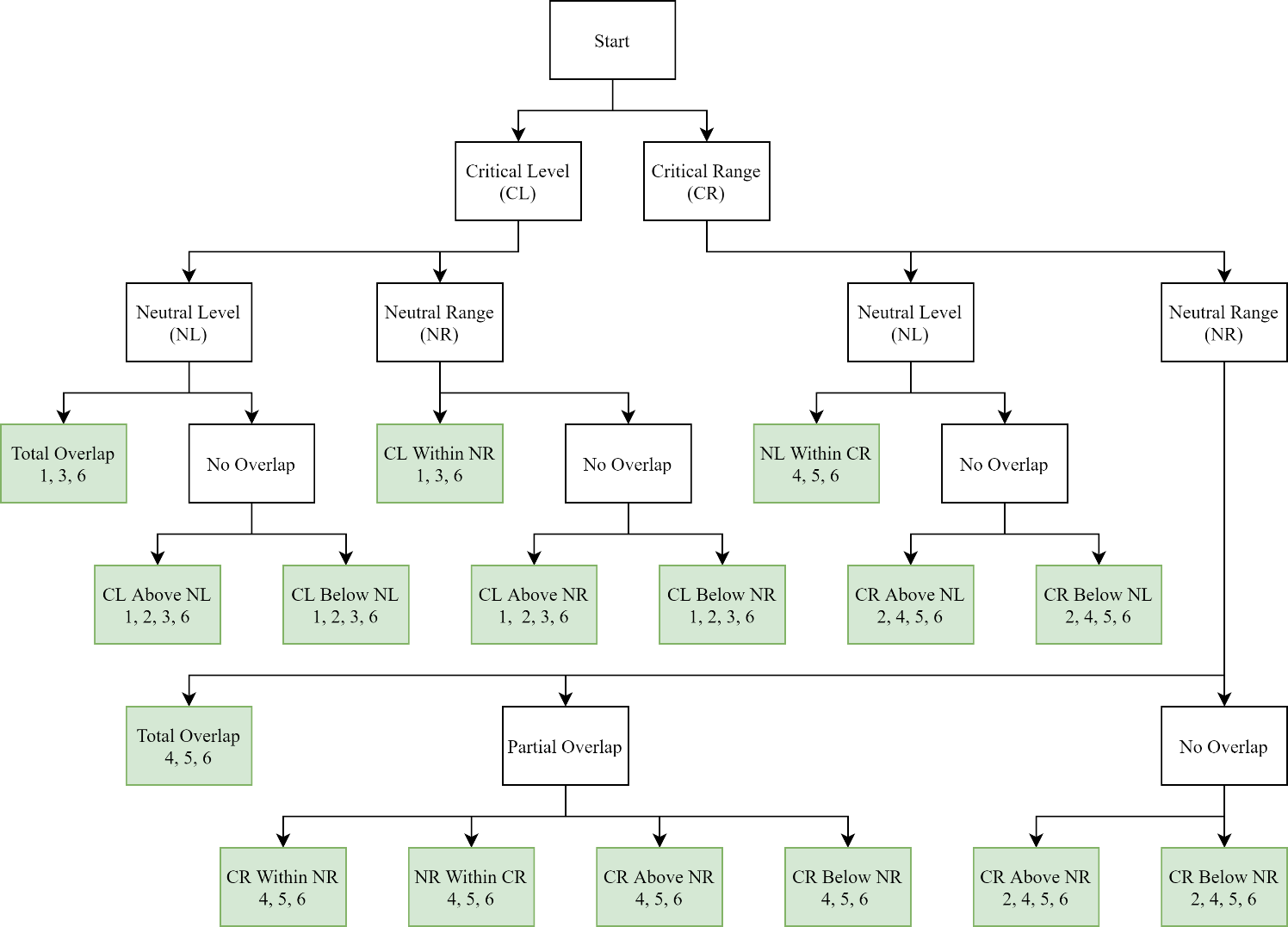
Many of the views in this taxonomy have never been advocated in print, but I lay them all out here for the sake of completeness. Four views that have been defended in print are the Total View, a positive critical-level view, a critical-range view, and a neutral-range view. I diagram them below. Horizontal lines denote that lives at the corresponding welfare level are personally/contributively strictly neutral. Boxes denote that lives at the corresponding welfare levels are personally/contributively weakly neutral. Lives at welfare levels above (below) the horizontal line or shaded box are personally/contributively good (bad). The numbers are purely illustrative.

First, the Total View (fig. 2), which is defended by Hudson (1987), Tännsjö (2002), and Huemer (2008), among others. There is a single coinciding neutral level and critical level, so that a life is personally good (bad/strictly neutral) iff it is contributively good (bad/strictly neutral). Any two populations are commensurable.

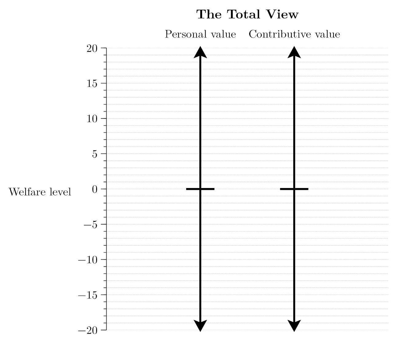
Second, a positive critical-level view (fig. 3), defended by Blackorby, Bossert, and Donaldson (2005) and Bossert (2022). There is a single critical level above a single neutral level, so a life can be personally good without being contributively good. Any two populations are commensurable.

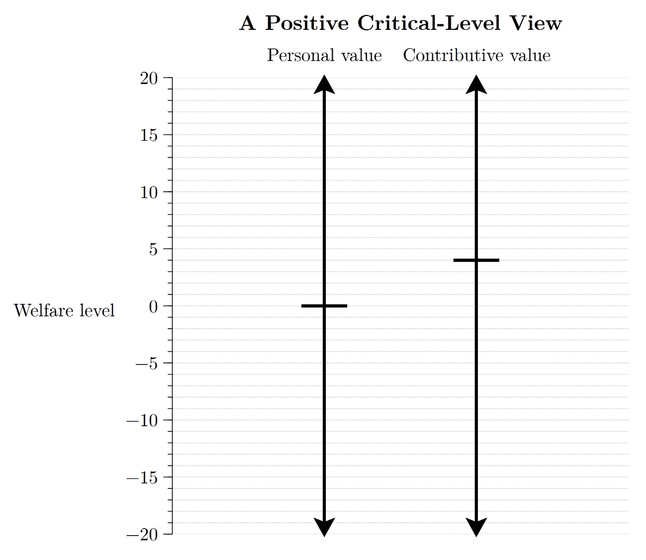
Third, a critical-range view. A view of this kind is defended by Broome (2004), who interprets the critical range as a range of indeterminacy, along with Qizilbash (2007; 2018) and Rabinowicz (2009), who each interpret the critical range as a range of parity. There is a single neutral level but a critical range, so any overlap between the neutral and critical sets can be partial at most. In figure 4, I present a version of the view in which the neutral level coincides with the lowest welfare level in the critical range. On critical-range views, some pairs of populations are incommensurable.

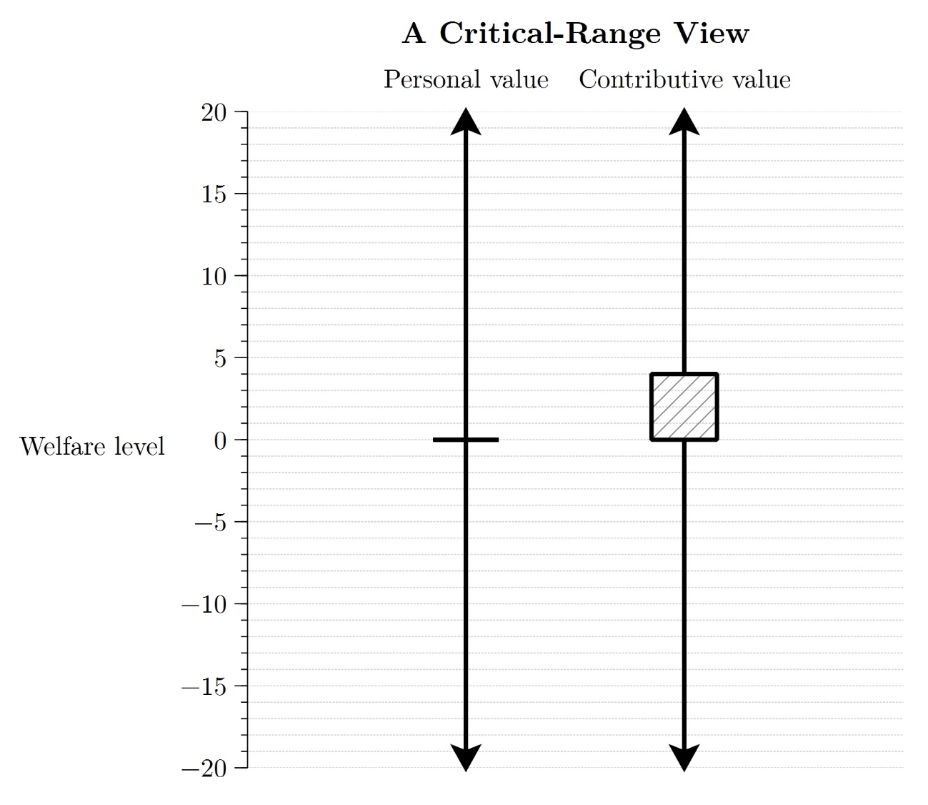
Finally, a neutral-range view (fig. 5). Rabinowicz (2020) discusses a view of this kind in more recent work, and Gustafsson (2020) defends a view of this form in which there is a neutral and critical range for temporal welfare levels as well as lifetime welfare levels. On neutral-range views, there is a neutral range and critical range that totally overlap, so a life is personally good (bad/weakly neutral) iff it is contributively good (bad/weakly neutral). Some pairs of populations are incommensurable.

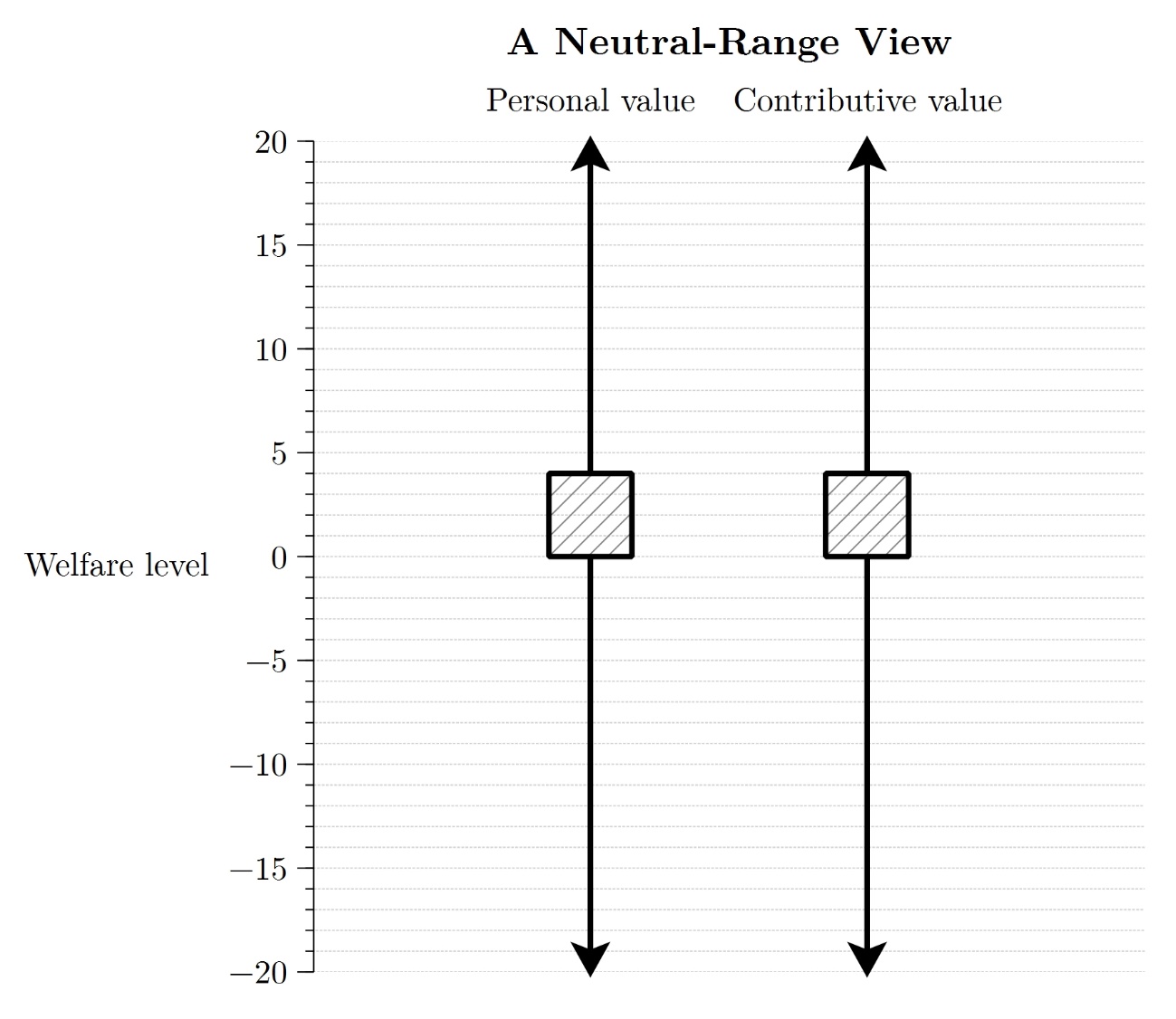
D. Objections to Critical-Set Views

Many varieties of critical-set view are subject to the same objections. Each view must reckon with at least three of the following six.

D.1. Maximal Repugnance

Any critical-set view on which lives barely worth living are contributively good will imply the:

Repugnant Conclusion: Each population of wonderful lives is worse than some population of lives barely worth living. (see Parfit 1984, 388)

And any critical-set view on which lives barely worth not living are contributively bad will imply the:

Mirrored Repugnant Conclusion: Each population of awful lives is better than some population of lives barely worth not living. (see Gustafsson 2020, 85)⁠Carlson (1998, 297) calls this claim the ‘Reverse Repugnant Conclusion’. Broome (2004, 213) calls it the ‘Negative Repugnant Conclusion’.

Both of these consequences arise because, on critical-set views, a population of enough contributively good (bad) lives can be better (worse) than any other population.

However, as Rabinowicz (2009, 406; 2020, 79) notes, the repugnance of these conclusions is attenuated if lives at a wide range of welfare levels are personally neutral. In that case, lives barely worth living are much better than lives barely worth not living. What makes the Repugnant Conclusion and its mirror troubling is the presumed similarity of lives barely worth living and lives barely worth not living. With that in mind, I define Maximal Repugnance as follows:

Maximal Repugnance: There is a life \(x\) and a life \(y\) that is identical but for one fewer gumdrop’s worth of pleasure and one more hangnail’s worth of pain such that (1) each population of wonderful lives is worse than some population of \(x\) lives and (2) each population of awful lives is better than some population of \(y\) lives.

Note that I drop the specification that \(x\) is barely worth living and \(y\) is barely worth not living. This feature is not necessary for repugnance. Suppose, for example, that we accept a view that implies Maximal Repugnance for a life \(x\) that is significantly personally good. This move mitigates the force of implication (1): we might be quite happy to accept that each population of wonderful lives is worse than some population of significantly personally good lives. But it exacerbates the implausibility of implication (2): if \(x\) is significantly personally good, then \(y\) is personally good, and it is hard to believe that each population of awful lives is better than some population of personally good lives. More generally, at least one of implications (1) and (2) will be implausible no matter how good \(x\) and \(y\) are.

Given that one fewer gumdrop’s worth of pleasure and one extra hangnail’s worth of pain can push a life’s welfare level from above the critical level to below it, all critical-level views imply Maximal Repugnance.

D.2. Sadism

Any view on which there is no overlap between the critical set and the neutral set implies some sadistic conclusion. If the critical set is above the neutral set and there is some welfare level between the two, the view implies the original:

Sadistic Conclusion: Each population of awful lives is better than some population of personally good lives. (see Arrhenius 2000a, 256)

That is because lives at a welfare level above the neutral set and below the critical set are personally good but contributively bad. And on critical-set views, adding enough contributively bad lives to a population can make that population worse than any other.

If the critical set is below the neutral set and there is some welfare level between them, the view implies the:

Mirrored Sadistic Conclusion: Each population of wonderful lives is worse than some population of personally bad lives. (see Gustafsson 2020, 85)

That is because lives at a welfare level below the neutral set and above the critical set are personally bad but contributively good. And on critical-set views, adding enough contributively good lives to a population can make that population better than any other.

We could endorse a critical-set view on which there is no overlap between the neutral set and the critical set and yet no welfare level between the two sets.⁠That is possible if welfare levels are not dense (by which I mean, there is some pair of distinct welfare levels with no welfare level between them) or if the neutral set and critical set are such that exactly one of them is open at the end where they meet (for example, if the neutral set is [0, 1) and the critical set is [1, 2]). These kinds of views imply only weaker forms of sadism. If the critical set is above the neutral set, the view implies a:

Weaker Sadistic Conclusion: Each population of awful lives is better than some population of personally neutral lives.

If the critical set is below the neutral set, the view implies a:

Weaker Mirrored Sadistic Conclusion: Each population of wonderful lives is worse than some population of personally neutral lives.

These conclusions are more plausible than the pair above, but that is faint praise. In fact, comparison with the previous subsection will show that they could equally be called Stronger Mirrored and Stronger Repugnant Conclusions, respectively.⁠I use the words ‘weaker’ and ‘stronger’ rather than ‘weak’ and ‘strong’ to distinguish these conclusions from the Weak Sadistic Conclusion and Strong Repugnant Conclusion that appear in Gustafsson (2020, 86) and Meacham (2012, 270) respectively.

All views with no overlap between the critical set and the neutral set imply some form of sadism.

D.3. Strong Superiority across Slight Differences

Consider a sequence of lives beginning with a contributively good life \(x_{1}\)⁠. We reach \(x_{2}\) by making \(x_{1}\) slightly worse. Perhaps \(x_{2}\) is identical to \(x_{1}\) but for one extra hangnail’s worth of pain. We reach \(x_{3}\) by making \(x_{2}\) slightly worse, and so on. After a finite number of slight detriments we reach \(x_{n}\)⁠, a contributively bad life.

On critical-level views, each life is either contributively good, contributively strictly neutral, or contributively bad. That means that, in our sequence, there is some contributively good life \(x_{k}\) such that \(x_{k + 1}\) is either contributively strictly neutral or contributively bad. That in turn implies that \(x_{k}\) has positive contributive value, while \(x_{k + 1}\)⁠’s contributive value is nonpositive. Adding positive numbers can never yield a nonpositive number, and vice versa, so critical-level views imply that any population of lives \(x_{k}\) is better than any population of lives \(x_{k + 1}\)⁠. Call this implication Strong Superiority across Slight Differences (SSASD).⁠For discussions of superiority and noninferiority in axiology, see Arrhenius and Rabinowicz (2015b), Nebel (2021), and Chapter 1 of this thesis.

We might claim that this implication is of little concern: \(x_{k}\) is contributively good and \(x_{k + 1}\) is not, so the strong superiority of \(x_{k}\) over \(x_{k + 1}\) should come as no surprise. But this level of description masks the difficulty. Consider a case in which each life in our \(x\)-sequence is long and turbulent, featuring soaring highs and crushing lows. Amid these peaks and troughs, we might expect a hangnail to pale almost into axiological insignificance. But critical-level views imply that this drop in the ocean can make all the difference: there will be a long, turbulent life \(x_{k}\) such that any population of lives \(x_{k}\) is better than any population of lives \(x_{k + 1}\) identical but for the extra hangnail. Two corollaries of this implication bring out its implausibility: a population of just a single life without the hangnail is better than any population of lives with it, and a population of just a single life with the hangnail is worse than any population of lives without it.

D.4. Strong Noninferiority across Slight Differences

This instance of SSASD might spur us to adopt a critical-range view. On critical-range views, lives at a range of welfare levels are contributively weakly neutral. If this range is wide enough, our \(x\)-sequence will contain no lives \(x_{k}\) and \(x_{k + 1}\) such that \(x_{k}\) is contributively good and \(x_{k + 1}\) is contributively strictly neutral or bad. If \(x_{k}\) is the last contributively good life in the sequence, then \(x_{k + 1}\) will be contributively weakly neutral. That means that critical-range views can avoid SSASD, because it is not the case that any population of contributively good lives is better than any population of contributively weakly neutral lives. Instead, each population of contributively good lives is incommensurable with some population of contributively weakly neutral lives. Here is an example to warm us up for the proof.

Suppose that all the welfare levels between 0 and 4 inclusive are critical. And suppose that \(w\left( x_{k} \right) = 4.01\) and \({w(x}_{k + 1}) = 3.99\)⁠. Population \(X\) consisting of a single life \(x_{k}\) is better than population \(Y\) consisting of a single life \(x_{k + 1}\)⁠, because \(v(X) > v(Y)\) for each critical level \(q\) in the critical set \(Q\)⁠. But \(X\) is incommensurable with population \(Z\) consisting of two lives \(x_{k + 1}\)⁠. \(X\) has greater value than \(Z\) relative to \(q = 4\)⁠, but \(Z\) has greater value than \(X\) relative to \(q = 0\)⁠.⁠\({v(X)}_{4} = (4.01 - 4) = 0.01\) and \({v(Z)}_{4}\)\(= (3.99 - 4)\)\(+ (3.99 - 4)\)\(= - 0.02\)⁠; \({v(X)}_{0} = (4.01 - 0) = 4.01\) and \({v(Z)}_{0}\)\(= (3.99 - 0)\)\(+ (3.99 - 0)\)\(= 7.98\)⁠.

More generally, each contributively weakly neutral life has positive contributive value relative to some critical level \(q\)⁠.⁠We might think that lives at the lowest welfare level in the critical range are a counterexample to this claim. They do not have positive value relative to any critical level \(q\) in the critical range \(Q\)⁠. But these lives are not contributively weakly neutral. On our definitions, they are contributively bad. Here is why. Suppose \(w(x)\) is the lowest welfare level in the critical range \(Q\)⁠. Then, for any population \(X\)⁠, the value of \(X\) is at least as great as the value of \(X\) plus a life at \(w(x)\) relative to each \(q\) in \(Q\)⁠, so \(X\) is at least as good as \(X\) plus a life at \(w(x)\)⁠. But the value of \(X\) plus a life at \(w(x)\) is not at least as great as the value of \(X\) relative to each \(q\) in \(Q\) (in particular, it is not at least as great relative to critical levels \(q\) that are not the lowest in the critical range), so \(X\) plus a life at \(w(x)\) is not at least as good as \(X\)⁠. Therefore, \(X\) plus a life at \(w(x)\) is worse than \(X\)⁠, and \(x\) is contributively bad. This is strange because \(w(x)\) is in the critical range, but this strangeness turns out to be of little consequence. We just need to bear in mind that only lives within the boundaries of the critical range are contributively weakly neutral. That implies that each population has less value than some sufficiently large population of contributively weakly neutral lives relative to that \(q\)⁠. Therefore, each population is not better than some sufficiently large population of contributively weakly neutral lives.

However, critical-range views still imply Strong Noninferiority across Slight Differences: for some \(x_{k}\) and \(x_{k + 1}\) in our \(x\)-sequence, any population of lives \(x_{k}\) is not worse than any population of lives \(x_{k + 1}\)⁠. To see how, return to our example above. No matter how many lives \(x_{k}\) are contained in \(X\)⁠, and no matter how many lives \(x_{k + 1}\) are contained in \(Z\)⁠, \(X\) will have greater value than \(Z\) relative to \(q = 4\)⁠. Therefore \(X\) is not worse than \(Z\)⁠, no matter what their respective sizes. More generally, for any contributively good life \(x_{k}\) and any contributively weakly neutral life \(x_{k + 1}\)⁠, there exists some \(q\) such that \(x_{k}\) has positive contributive value relative to \(q\) and \(x_{k + 1}\) has nonpositive contributive value relative to \(q\)⁠. So relative to this \(q\)⁠, any population of lives \(x_{k}\) has greater value than any population of lives \(x_{k + 1}\)⁠. That in turn implies that any population of lives \(x_{k}\) is not worse than any population of lives \(x_{k + 1}\). This kind of discontinuity is innocuous considered in itself. But as I demonstrate below, critical-range views imply that Strong Noninferiority across Slight Differences occurs in some counterintuitive places.

Consider a new sequence. Each life in this sequence features a blank period, free of any good or bad components. We can imagine it as a minute of dreamless sleep. The first life in the sequence \(y_{0}\) also features a period of constant happiness of length \(n\) hours, and nothing else. The second life \(y_{1}\) is identical, except that the happiness lasts \(n - 1\) hours. \(y_{2}\)⁠’s happiness lasts \(n - 2\) hours, and so on. Call all such lives featuring only good and neutral components straightforwardly-better-than-blank. Life \(y_{n}\) features only the blank period and so qualifies as a blank life, featuring no good or bad components whatsoever (Broome 2004, 208). Life \(y_{n + 1}\) features the blank period plus one hour of suffering, \(y_{n + 2}\) features the blank period plus two hours of suffering, and so on. The last life in the sequence is \(y_{2n}\)⁠, featuring the blank period plus \(n\) hours of suffering. Call all such lives featuring only bad and neutral components straightforwardly-worse-than-blank.

Intuitively, the first discontinuity in this sequence occurs between \(y_{n - 1}\) and \(y_{n}\)⁠. That is, \(y_{n - 1}\) is strongly noninferior to \(y_{n}\)⁠: any population of lives \(y_{n - 1}\) featuring one hour of happiness is not worse than any population of blank lives \(y_{n}\)⁠. And, again intuitively, the second discontinuity in this sequence occurs between \(y_{n}\) and \(y_{n + 1}\)⁠. That is, \(y_{n + 1}\) is strongly nonsuperior to \(y_{n}\)⁠: any population of lives \(y_{n + 1}\) featuring one hour of suffering is not better than any population of blank lives \(y_{n}\)⁠. These two claims remain intuitive when we replace ‘hours’ with ‘minutes,’ ‘seconds,’ ‘milliseconds,’ and so on.

But critical-range views must deny at least one of these claims. Recall that on critical-range views, more than one welfare level is critical. Therefore, in any sequence with sufficiently small differences in welfare between adjacent lives, more than one life is contributively weakly neutral. We can make the differences in welfare between adjacent lives in our \(y\)-sequence arbitrarily small by replacing hours with smaller units of time, so for some such unit, more than one life in our \(y\)-sequence is contributively weakly neutral.

Suppose for illustration that when the unit of time is seconds, \(y_{n - 1}\) and \(y_{n}\) are the contributively weakly neutral lives. In that case, \(y_{n - 2}\) (the last contributively good life) is strongly noninferior to \(y_{n - 1}\) (the first contributively weakly neutral life). In other words, any population of lives featuring two seconds of happiness is not worse than any population of lives featuring one second of happiness. That implies that a population of just a single life featuring two seconds of happiness is not worse than any population of lives featuring one second of happiness. But this consequence seems implausible. The only difference between the lives is the duration of happiness; the latter population can feature an arbitrarily longer total duration of happiness; and yet the latter population can never be better than the former.

We get a mirror of this implication if we suppose instead that \(y_{n}\) and \(y_{n + 1}\) are the contributively weakly neutral lives. In that case, any population of lives featuring two seconds of suffering is not better than any population of lives featuring one second of suffering. Though this latter population can feature an arbitrarily longer total duration of suffering, it can never be worse than a population of just a single life featuring two seconds of suffering. This too seems implausible.

Nothing hinges on the particular lives chosen to illustrate this dynamic. Any critical-range view will imply that (1) a population of just a single straightforwardly-better-than-blank life is not worse than any population of straightforwardly-better-than-blank lives identical but for a slightly smaller quantity of good, or (2) a population of just a single straightforwardly-worse-than-blank life is not better than any population of straightforwardly-worse-than-blank lives identical but for a slightly smaller quantity of bad.

D.5. Maximal Greediness

Critical-range views face another difficulty. As Broome (2004, 169–70, 202–5) points out, they imply that contributively weakly neutral lives can ‘swallow up’ and neutralize goodness and badness. Here is an illustration of what that means. Suppose again that all welfare levels between 0 and 4 inclusive are critical. And suppose that population \(A\) consists of a single life \(x\) at welfare level 20. We reach population \(B\) by making two changes. We reduce \(x\)⁠’s welfare level by 1 and add a life \(y\) at welfare level 2. The combined effect of these changes might seem bad. We made one person worse off and added a life that is contributively weakly neutral. But our critical-range view implies that these changes are not bad. Neither \(A\)*‘s* nor \(B\)⁠’s value is at least as great as the other relative to each \(q\) in \(Q\)⁠, so the two populations are incommensurable.⁠Relative to \(q = 4\)⁠, \({v(A)}_{4} = (20 - 4) = 16\) and \({v(B)}_{4} = (19 - 4) + (2 - 4) = 13\)⁠. Relative \(q = 0\)⁠, \({v(A)}_{0} = (20 - 0) = 20\) and \({v(B)}_{0} = (19 - 0) + (2 - 0) = 21\)⁠. Our critical-range view also implies that \(A\) is incommensurable with \(C\) (in which \(x\)⁠’s welfare level is 18 and there are two lives at welfare level 2) and \(D\) (in which \(x\)⁠’s welfare level is 17 and there are three lives at welfare level 2) and so on. This process can continue indefinitely. \(A\) will also be incommensurable with a population \(Z\)⁠, in which \(x\)⁠’s welfare level is extremely low and there is some large number of contributively weakly neutral lives. Broome and I find this ’greedy neutrality’ concerning, but others are happy to bite the bullet (Rabinowicz 2009; Frick 2017; Gustafsson 2020). In any case, the worry can be sharpened.

Note first that the size of population \(A\) need not be restricted to a single life: adding enough contributively weakly neutral lives can neutralize any finite loss of welfare for existing people. And suppose that blank lives are contributively weakly neutral. In that case, for any arbitrarily good population and any arbitrarily bad population, there is some population of blank lives—featuring no good or bad components whatsoever—such that the good population plus the blank lives is not better than the bad population. This implication seems difficult to accept.

It gets worse. Consider again our \(y\)-sequence above. Given that the unit of time is sufficiently small, critical-range views imply that more than one life in this sequence is contributively weakly neutral. For illustration, suppose that the blank life \(y_{n}\) and the straightforwardly-better-than-blank life \(y_{n - 1}\) are contributively weakly neutral. In that case, we can replace ‘blank lives’ with ‘straightforwardly-better-than-blank lives’ in the above paragraph. For any arbitrarily good population and any arbitrarily bad population, there is some population of straightforwardly-better-than-blank lives—featuring no bad components whatsoever and some happiness—such that the good population plus the straightforwardly-better-than-blank lives is not better than the bad population. The former population might feature only neutral and good components; the latter population might feature only bad components; and yet this critical-range view implies that the former is not better than the latter.

If the straightforwardly-worse-than-blank life \(y_{n + 1}\) is contributively weakly neutral, we get a mirror of this implication. For any arbitrarily good population and any arbitrarily bad population, there is some population of straightforwardly-worse-than-blank lives—featuring no good components whatsoever and some suffering—such that the bad population plus the straightforwardly-worse-than-blank lives is not worse than the good population. Call implications of this kind Maximal Greediness.

Shifting the critical range away from blank lives fails to mitigate the difficulty. If the critical range is above or below the welfare level of a blank life, then some other life in our \(y\)-sequence will be contributively weakly neutral. No matter where the critical range is placed, we get Maximal Greediness.

D.6. No Incommensurability between Lives or between Same-Size Populations

On critical-level views, a population’s value can be represented by a real number. Since any two real numbers are commensurable (\(a\) is at least as great as \(b\) or \(b\) is at least as great as \(a\)⁠), critical-level views imply that any two populations are commensurable: \(X\) is at least as good as \(Y\) or \(Y\) is at least as good as \(X\)⁠.

However, universal commensurability seems implausible. Consider the following small improvement argument (De Sousa 1974; Chang 2002). Suppose that \(X\) consists of 10 wonderful lives and \(Y\) consists of 100 very good lives. Neither \(X\) nor \(Y\) is better than the other.⁠Those who disagree should tweak the numbers or adjectives. If any two populations are commensurable, \(X\) and \(Y\) are equally good. But if \(X\) and \(Y\) are equally good, then any population better than \(Y\) is better than \(X\)⁠. \(Y^{+}\)⁠, consisting of 100 slightly-better-than-very-good lives, is better than \(Y\) but not better than \(X\)⁠. Therefore, \(X\) and \(Y\) are not equally good. They are incommensurable.

Critical-range views can account for this incommensurability. They can claim that \(X\) has greater value than \(Y\) relative to one level in the critical range and that \(Y\) has greater value than \(X\) relative to another level. But this explanation cannot account for all plausible instances of incommensurability. In particular, it cannot account for the incommensurability of same-size populations.

This is easiest to see in the single-life case. Critical-set views assume that a life’s welfare can be represented by a real number. Since any two real numbers are commensurable, this assumption implies that any two lives are commensurable: \(x\) is at least as good as \(y\) or \(y\) is at least as good as \(x\)⁠.

Now note critical-set views’ equation for the value of a population \(X\) relative to a critical level \(q\)⁠:

\[{v(X)}_{q} = \sum_{i}^{}{(w\left( x_{i} \right) - q)}\](69)

Since this equation is a sum of welfare levels minus the critical level, assuming that a life’s welfare can be represented by a real number implies that a population’s value relative to a critical level can be represented by a real number. That in turn implies that the value of any two populations relative to a critical level is commensurable. Formally,

(1) For any populations \(X\) and \(Y\) and any critical level \(q\)⁠, \({v(X)}_{q} \geq {v(Y)}_{q}\) or \({v(Y)}_{q} \geq {v(X)}_{q}\)⁠.

Now let \(X\) and \(Y\) stand for arbitrary same-size populations and \(q\) stand for an arbitrary critical level such that \({v(X)}_{q} \geq {v(Y)}_{q}\)⁠. Substituting in the equations for \({v(X)}_{q}\) and \({v(Y)}_{q}\) gives us the following inequality:

\[\sum_{i}^{}{(w\left( x_{i} \right) - q)} \geq \sum_{i}^{}{(w\left( y_{i} \right) - q)}\](70)

This inequality can also be expressed as follows, with \(n\) representing the size of populations \(X\) and \(Y\)⁠:

\[\left( \sum_{i}^{}{w\left( x_{i} \right)} \right) - nq \geq \left( \sum_{i}^{}{w\left( y_{i} \right)} \right) - nq\](71)

The terms involving \(q\) can then be canceled from each side:

\[\sum_{i}^{}{w\left( x_{i} \right)} \geq \sum_{i}^{}{w\left( y_{i} \right)}\](72)

Therefore, the inequality is true for all values of \(q\)⁠, and \(X\) is at least as good as \(Y\)⁠. Since \(X\)⁠, \(Y\)⁠, and \(q\) were arbitrary, we can conclude:

(2) For any same-size populations \(X\) and \(Y\) and any critical level \(q\)⁠, if \({v(X)}_{q} \geq {v(Y)}_{q}\)⁠, then \(X\) is at least as good as \(Y\)⁠.

Together, (1) and (2) imply:

(3) For any same-size populations \(X\) and \(Y\)⁠, \(X\) is at least as good as \(Y\) or \(Y\) is at least as good as \(X\)⁠.

In other words, critical-set views imply that any two same-size populations are commensurable.

However, universal commensurability of same-size populations seems implausible. Consider another small improvement argument. Suppose that \(x\) is a turbulent life, featuring soaring highs and crushing lows, and that \(y\) is a drab life, featuring only Muzak and potatoes (Parfit 1986, 148). If we fix the relative quantities of \(x\)⁠’s highs and lows in the right way, neither \(x\) nor \(y\) is better than the other. Yet \(x\) and \(y\) cannot be equally good because a slightly less drab life \(y^{+}\)—featuring Muzak, potatoes, and ketchup—is better than \(y\) but not better than \(x\)⁠. Therefore, \(x\) and \(y\) are incommensurable. Similar arguments suggest the incommensurability of other pairs of same-size populations.

Partly on the basis of such arguments, advocates of critical-set views have started to incorporate incommensurability and indeterminacy into their theories of personal betterness. Broome (2022), for example, states that some pairs of lives are obviously indeterminately related but offers no explanation for why this is so. Rabinowicz (2020), meanwhile, offers a fitting-attitudes analysis of parity—one species of incommensurability—according to which two lives are on a par iff it is permissible to prefer either life to the other. And Gustafsson (2020) accounts for incommensurability between lives by claiming that there is a neutral range of temporal welfare levels. Adding a moment within this range to a life renders the new life incommensurable with the original.

Gustafsson’s move strikes me as a step in the right direction. However, his view cannot account for the incommensurability between same-length lives for the same reason that critical-range views cannot account for the incommensurability between same-size populations. Gustafsson might claim that any two lives of the same length are commensurable, but this claim seems implausible. The small improvement argument involving drab and turbulent lives remains convincing if we specify that the lives are the same length.

Rabinowicz’s (2020, 81) account is incomplete but, I believe, more promising. He claims that ‘life wellbeing is a many-dimensional concept,’ that ‘specifying its level requires characterizing a life with respect to several relevant dimensions,’ and that ‘different weight assignments’ to these relevant dimensions give rise to incommensurability between lives. This notion of ‘different weight assignments’ forms the core of the Imprecise Exchange Rates View.

E. Imprecise Exchange Rates

Some trade-offs are worth making. For example, going to the dentist to prevent tooth decay is a trade-off worth making. The good of having healthy teeth outweighs the bad of the trip. Other trade-offs are worth not making. Getting up at 4 a.m. and walking to work to save the £2 bus fare is a trade-off worth not making. The bad outweighs the good. Still other trade-offs are neither worth making nor worth not making, and a small improvement fails to break the deadlock. Here is an example.

A parent says to their child, ‘No dessert unless you finish your dinner.’ The child knows exactly what finishing dinner involves. They are all too familiar with the taste of peas and can see one hundred of them left on the plate. They also know what dessert will be like. The jelly is sitting on the counter and promises to taste as good as it always has. In this case, the trade-off may be neither worth making nor worth not making. And a small improvement to the child’s predicament need not resolve the issue. Suppose that the parent takes pity on the child and removes one pea from the plate. That need not ensure that finishing dinner is now a trade-off worth making.

I claim that cases of this kind are evidence that various exchange rates—between pairs of goods, between pairs of bads, and between goods and bads—are imprecise. This imprecision renders certain goods incommensurable with other goods, certain bads incommensurable with other bads, and certain combinations of goods and bads incommensurable with other combinations. In the child’s case, eating both the peas and the jelly is incommensurable with eating neither. This incommensurability between goods, bads, and their combinations is the source of incommensurability between lives. The child’s life in which they eat the peas and jelly is incommensurable with the otherwise identical life in which they eat neither.

That is one motivation for the Imprecise Exchange Rates (IER) View. Now for the formalization. Recall that critical-set views begin with an ordering of lives by welfare. The IER View begins instead with a set of orderings: one for each dimension of good and bad within a life. The exact form of the view thus depends on our theory of welfare. If we accept the simplest hedonist theory, there are just two orderings: one of happiness and one of suffering. If we accept an objective list theory, there are more orderings: perhaps one of love, one of virtue, one of false belief, etc. Welfare levels are thus given by vectors. Suppose, for example, that we accept an objective list theory on which happiness (\(h\)⁠), love (\(l\)⁠), suffering (\(s\)⁠), and false belief (\(f)\) are the dimensions of good and bad. Then the welfare level of a life \(x\) is as follows:

\[w(x) = \left\langle h(x),\ l(x),\ s(x),\ f(x) \right\rangle\](73)

I assume that \(h\)⁠, \(l\)⁠, \(s\)⁠, and \(f\) are real-valued functions. I also assume that the values of each function are interpersonally level-comparable (so that we can make claims like ‘The life Ada would have as an artist features more happiness than the life Bob would have as a baker.’) and measurable on a ratio scale (so that we can make claims like ‘The life Ada would have as an artist features twice the suffering of the life Ada would have as a baker.’). Blank lives—featuring no good or bad components whatsoever—score 0 on each dimension.

Each ratio scale is independent, so we cannot yet compare values across dimensions. We cannot make claims like ‘In the life Ada would have as an artist, her happiness outweighs her suffering.’ Comparisons of this kind are only possible given a specified proto-exchange-rate \(r\)⁠: a vector of two or more real numbers strictly greater than 0 and summing to 1 denoting the relative weight granted to each dimension of good and bad. On the objective list theory above, for example, each proto-exchange-rate \(r\) will take the form \(\left\langle r_{h},\ r_{l},\ r_{s},\ r_{f} \right\rangle\)⁠, where \(r_{h}\) denotes the weight granted to happiness, \(r_{l}\) denotes the weight granted to love, and so on. Letting \(x\) represent the life Ada would have as an artist, the claim that her happiness outweighs her suffering relative to a given \(r\) will be true iff

\(r_{h}h(x) > r_{s}s(x)\)⁠.

On the IER View, only welfare levels relative to a given \(r\) can be expressed as a real number. Continuing with our example objective list theory, the equation is as follows:

\[{w(x)}_{r} = r_{h}h(x) + r_{l}l(x) - r_{s}s(x) - r_{f}f(x)\](74)

The value of a population relative to \(r\) is the sum of the welfare levels of each of its lives relative to \(r\)⁠:

\[{v(X)}_{r} = \sum_{i}^{}{w\left( x_{i} \right)}_{r}\](75)

We then account for incommensurability by claiming that there are multiple proto-exchange-rates \(r\) in the set of all admissible proto-exchange-rates \(R\)⁠. A life \(x\) is at least as good as a life \(y\) iff \({w(x)}_{r} \geq {w(y)}_{r}\) relative to each \(r\) in \(R\)⁠. And a population \(X\) is at least as good as a population \(Y\) iff \({v(X)}_{r} \geq {v(Y)}_{r}\) relative to each \(r\) in \(R\)⁠.⁠Rabinowicz (2020, 83–84) offers a similar formalization. His formalization, however, takes a set of permissible preferential ratio scales over the set of lives as primitive. It does not specify how the dimensions of welfare weigh against each other.

In what follows, I mostly discuss a simple hedonist version of the IER View, in which the welfare level of a life \(x\) is given by a vector of happiness and suffering, \(\left\langle h(x),\ s(x) \right\rangle\)⁠, with the functions \(h\) and \(s\) normalized so that the proto-exchange-rate \(r\) composed of \(r_{h} = 0.5\) and \(r_{s} = 0.5\) falls within the set \(R\)⁠. I adopt hedonism purely for the sake of simplicity. Its two dimensions are sufficient to illustrate the most important advantages and drawbacks of the IER View. My discussion below applies equally to variants of the view with more dimensions.

F. Advantages of the Imprecise Exchange Rates View

The IER View has several advantages over critical-set views. Here are four.

F.1. Some Incommensurability between Lives and between Same-Size Populations

The first advantage is that the IER View offers a simple and plausible account of incommensurability between lives and between same-size populations. Recall that a life is at least as good as another iff its welfare level is at least as great relative to each \(r\) in \(R\)⁠. If \(R\) contains more than one \(r\)⁠, then some pairs of lives are incommensurable: neither is at least as good as the other.

Consider an example. Suppose that \(R\) contains each \(r\) in which \(0.4 \leq r_{h} \leq 0.6\)⁠. Since \(r_{h} + r_{s} = 1\)⁠, \(r_{s} = 1 - r_{h}\)⁠. In that case, life \(x\)—at welfare level \(\left\langle 4,\ 1 \right\rangle\)—is incommensurable with life \(y\)—at welfare level \(\left\langle 10,\ 6 \right\rangle\)⁠. The welfare level of \(x\) is greater relative to \(r_{h} = 0.4\)⁠, but the welfare level of \(y\) is greater relative to \(r_{h} = 0.6\)⁠.⁠\({w(x)}_{r_{h} = 0.4}\)\(= 0.4 \times 4 - 0.6 \times 1\)\(= 1\) and \({w(y)}_{r_{h} = 0.4}\)\(= 0.4 \times 10 - 0.6 \times 6\)\(= 0.4\)⁠; \({w(x)}_{r_{h} = 0.6}\)\(= 0.6 \times 4 - 0.4 \times 1\)\(= 2\) and \({w(y)}_{r_{h} = 0.6}\)\(= 0.6 \times 10 - 0.4 \times 6\)\(= 3.6\)⁠. This is as it should be. Taking on the extra suffering in \(y\) for the sake of the extra happiness is a trade-off neither worth making nor worth not making.

The IER View also gives us the right result in small improvement cases. A slightly improved life \(y^{+}\) at welfare level \(\left\langle 10 + e,\ 6 \right\rangle\) comes out better than \(y\) and incommensurable with \(x\)⁠. That is because the IER View accounts for the incommensurability between lives while respecting a certain kind of dominance:

Dominance over Dimensions: For any lives \(x\) and \(y\) and any set of proto-exchange-rates \(R\)⁠, if for each good dimension \(g\)⁠, \(x\) features at least as much \(g\) as \(y\)⁠, and for each bad dimension \(b\)⁠, \(x\) features at most as much \(b\) as \(y\)⁠, \(x\) is at least as good as \(y\)⁠. If, in addition, \(x\) features more \(g\) than \(y\) for some \(g\) or less \(b\) than \(y\) for some \(b\)⁠, \(x\) is better than \(y\)⁠.⁠Here is a sketch of the proof. Life \(x\) is at least as good as life \(y\) relative to any \(R\) iff \(r_{h}h(x) - r_{s}s(x) \geq r_{h}h(y) - r_{s}s(y)\) for any \(0 < r_{h} < 1\) and \(r_{s} = 1 - r_{h}\)⁠. Rearranging this equation gives \(r_{h}\left( h(x) - h(y) \right)\)\(+ r_{s}\left( s(y) - s(x) \right) \geq 0\)⁠. If \(x\) dominates \(y\)⁠, then \(h(x) \geq h(y)\) and \(s(y) \geq s(x)\)⁠, so each term on the left-hand side of the inequality in the previous sentence is nonnegative. Therefore, the weak inequality holds. If, in addition, \(x\) features more happiness or less suffering than \(y\)⁠, then at least one term on the left-hand side of the inequality is positive, so the strict inequality holds. This proof can be extended to any number of dimensions of good and bad.

Another implication is related. Let us say that two proto-exchange-rates differ in optimism iff they differ in the total weight granted to all dimensions of good taken together.⁠Here is an example. Return briefly to our objective list theory on which happiness, love, suffering, and false belief are the dimensions of good and bad, and consider the following three proto-exchange-rates: \(r_{1}\)\(= \left\langle 0.3,\ 0.2,\ 0.1,\ 0.4 \right\rangle\)⁠, \(r_{2}\)\(= \left\langle 0.2,\ 0.3,\ 0.1,\ 0.4 \right\rangle\)⁠, and \(r_{3}\)\(= \left\langle 0.3,\ 0.3,\ 0.1,\ 0.3 \right\rangle\)⁠. Proto-exchange-rates \(r_{1}\) and \(r_{2}\) are distinct because \(r_{1}\) assigns more weight to happiness while \(r_{2}\) assigns more weight to love. But they are equally optimistic because they both assign a weight of 0.5 to both dimensions of good taken together. Proto-exchange-rate \(r_{3}\)⁠, meanwhile, differs in optimism from both \(r_{1}\) and \(r_{2}\) because \(r_{3}\) assigns a weight of 0.6 to both dimensions of good taken together. The implication is that if \(R\) contains proto-exchange-rates that differ in optimism, then only lives featuring identical quantities of good and bad can be equally good.⁠To see this result, note first that equally good lives must have the same welfare level relative to each proto-exchange-rate. If \(x\) has a greater welfare level than \(y\) relative to some proto-exchange-rate, \(y\) is not at least as good as \(x\)⁠, and so the pair cannot be equally good. Now let \(g(x)\) denote the total quantity of good in \(x\)⁠, \(b(x)\) denote the total quantity of bad in \(x\)⁠, and so on, and let \(r_{1}\) and \(r_{2}\) denote the total weight assigned to dimensions of good relative to proto-exchange-rates that differ in optimism. If \(x\) and \(y\) are equally good, then \(r_{1}g(x) - (1 - r_{1})b(x)\)\(= r_{1}g(y) - (1 - r_{1})b(y)\) and mutatis mutandis for \(r_{2}\)⁠. Rearranging these equations gives \(r_{1}\left( g(x) - g(y) + b(x) - b(y) \right)\)\(+ b(x) - b(y)\)\(= 0\) and mutatis mutandis for \(r_{2}\)⁠. Since both expressions equal \(0\)⁠, they equal each other. Canceling \(b(x) - b(y)\) from each side gives \(r_{1}\left( g(x) - g(y) + b(x) - b(y) \right)\)\(= r_{2}\left( g(x) - g(y) + b(x) - b(y) \right)\)⁠. Since \(r_{1} \neq r_{2}\)⁠, the expression \(g(x) - g(y) + b(x) - b(y)\) must equal \(0\)⁠. That is true iff there exists some \(k\) such that \(g(x) - g(y) = k\) and \(b(x) - b(y) = - k\)⁠. If \(k > 0\)⁠, then \(g(x) > g(y)\) and \(b(x) < b(y)\)⁠. In that case, \(x\) is better than \(y\) by strict dominance, so they cannot be equally good. If \(k < 0\)⁠, then \(y\) is better than \(x\) by strict dominance. The only remaining possibility is that \(k = 0\)⁠, in which case \(g(x) = g(y)\) and \(b(x) = b(y)\)⁠. Therefore, \(x\) and \(y\) are equally good only if they feature identical quantities of good and bad. That means that lives at welfare levels such as \(\langle 4,\ 4\rangle\) and \(\langle 5,\ 5\rangle\) come out incommensurable on the IER View. This result is exactly what we want. Undergoing the extra suffering for the sake of the extra happiness is a trade-off neither worth making nor worth not making. If lives at \(\langle 4,\ 4\rangle\) and \(\langle 5,\ 5\rangle\) were judged equally good, the view would generate counterintuitive verdicts in small improvement cases. For example, a life at \(\langle 4,\ 4\rangle\) would be worse than a life at \(\langle 5,\ 5 - e\rangle\) for any \(e > 0\)⁠. From now on, I assume that \(R\) contains proto-exchange-rates that differ in optimism.

The above three points are true of populations as well as lives. If \(R\) contains more than one \(r\)⁠, then some pairs of populations (including same-size populations) are incommensurable. If one population weakly (strictly) dominates another over dimensions, then it is at least as good (better). And if \(R\) contains proto-exchange-rates that differ in optimism, then only populations featuring identical quantities of good and bad can be equally good.

F.2. No Sadism

Recall that critical-set views positing no overlap between the critical set and the neutral set imply some sadistic conclusion: either each population of awful lives is better than some population of lives that are not personally bad, or each population of wonderful lives is worse than some population of lives that are not personally good.

The IER View can avoid this drawback. More precisely, the IER View avoids sadism if we make the plausible claim that blank lives are personally strictly neutral. This claim implies that only blank lives are personally strictly neutral since, as we saw in the last subsection, no lives differing in their quantities of good or bad can be equally good. The extension of personal strict neutrality then matches the extension of contributive strict neutrality since, on the IER View, only blank lives are contributively strictly neutral. Adding any other kind of life changes the quantity of good or bad in the population, and no populations differing in their quantities of good or bad can be equally good.

This coincidence of personal and contributive strict neutrality suffices to establish that each category of personal value coincides with the corresponding category of contributive value. That is because the IER View then determines each life’s personal and contributive category in the same way: its value is compared to the value of a blank life relative to each proto-exchange-rate in \(R\)⁠. That implies that a life is personally good (bad/strictly neutral/weakly neutral) iff it is contributively good (bad/strictly neutral/weakly neutral). Therefore, the IER View avoids all instances of sadism.

With the coincidence of each personal and contributive category of value on the IER View established, I often drop the words ‘personal’ and ‘contributive’ in what follows. In figure 6, I graph these coincident categories for lives at different welfare levels on the IER View with \(0.4 \leq r_{h} \leq 0.6\)⁠. A life is good (bad/weakly neutral) iff the point picked out by its quantity of suffering on the horizontal axis and its quantity of happiness on the vertical axis falls within the green (red/white) region. Lives at the origin are blank and hence strictly neutral.

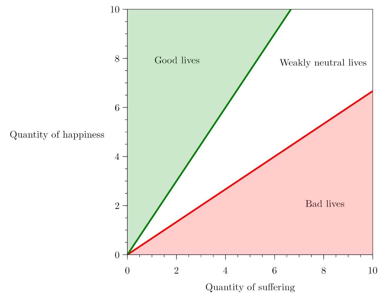
F.3. Less Concerning Superiority and Noninferiority

As we saw above, critical-level views imply a concerning instance of Strong Superiority across Slight Differences (SSASD) in our \(x\)-sequence: there exists some long, turbulent life \(x_{k}\) such that any population of lives \(x_{k}\) is better than any population of lives \(x_{k + 1}\) identical but for an extra hangnail. Critical-range views, meanwhile, imply only Strong Noninferiority across Slight Differences in our \(x\)-sequence: there exists some long, turbulent life \(x_{k}\) such that any population of lives \(x_{k}\) is not worse than any population of lives \(x_{k + 1}\) identical but for an extra hangnail. But on critical-range views, at least one discontinuity of this kind must occur in a counterintuitive place in our \(y\)-sequence, so that there exists some life \(y_{k}\) featuring only neutral components and happiness such that a population of just a single life \(y_{k}\) is not worse than any population of lives each featuring a slightly shorter duration of happiness, or there exists some life \(y_{j}\) featuring only neutral components and suffering such that a population of just a single life \(y_{j}\) is not better than any population of lives each featuring a slightly shorter duration of suffering.

The IER View avoids both of these problems. Consider first SSASD. Suppose, for illustration, that an extra hangnail adds 0.02 to a life’s quantity of suffering. Suppose also that some turbulent life \(x_{k}\) has welfare level \(\left\langle 9,\ 9 \right\rangle\)⁠. Life \(x_{k + 1}\) then has welfare level \(\left\langle 9,\ 9.02 \right\rangle\)⁠. Since \(x_{k}\) dominates \(x_{k + 1}\)⁠, population \(X\) consisting of a single life \(x_{k}\) is better than population \(Y\) consisting of a single life \(x_{k + 1}\)⁠. But \(X\) is incommensurable with population \(Z\)⁠, consisting of two lives \(x_{k + 1}\)⁠. \(X\) has greater value than \(Z\) relative to \(r_{h} = 0.4\)⁠, but \(Z\) has greater value than \(X\) relative to \(r_{h} = 0.6\)⁠.⁠\({v(X)}_{r_{h} = 0.4}\)\(= 0.4 \times 9 - 0.6 \times 9\)\(= - 1.8\) and \({v(Z)}_{r_{h} = 0.4}\)\(= (0.4 \times 9 - 0.6 \times 9.02)\)\(+ (0.4 \times 9 - 0.6 \times 9.02)\)\(= - 3.624\)⁠; \({v(X)}_{r_{h} = 0.6}\)\(= 0.6 \times 9 - 0.4 \times 9\)\(= 1.8\) and \({v(Z)}_{r_{h} = 0.6}\)\(= (0.6 \times 9 - 0.4 \times 9.02)\)\(+ (0.6 \times 9 - 0.4 \times 9.02)\)\(= 3.584\)⁠.

We get the same result with lives at many other welfare levels. In fact, the IER View avoids SSASD in all but a small minority of cases. To see those cases in which SSASD is implied, let \(\left\langle {h(x}_{k}),\ {s(x}_{k}) \right\rangle\) and \(\left\langle {h(x}_{k}),\ {s(x}_{k}) + 0.02 \right\rangle\) be the welfare levels of \(x_{k}\) and \(x_{k + 1}\) respectively. Life \(x_{k}\) is strongly superior to life \(x_{k + 1}\) iff \(x_{k}\) is good and \(x_{k + 1}\) is strictly neutral or bad, or \(x_{k}\) is strictly neutral and \(x_{k + 1}\) is bad. This condition is satisfied iff \(x_{k}\)⁠’s welfare level is nonnegative relative to the most pessimistic proto-exchange-rate \(r_{h} = 0.4\), \(x_{k + 1}\)⁠’s welfare level is nonpositive relative to the most optimistic proto-exchange-rate \(r_{h} = 0.6\), and at least one of \(x_{k}\)⁠’s or \(x_{k + 1}\)⁠’s welfare levels is non-zero relative to some \(r\) in \(R\).⁠The hangnail’s worth of pain ensures that this last condition is met. That yields two inequalities: \(0.4{h(x}_{k}) - 0.6{s(x}_{k}) \geq 0\) and \(0.6{h(x}_{k}) - 0.4\left( {s(x}_{k} \right) + 0.02) \leq 0\)⁠. Plotting these two inequalities gives us the region in figure 7.

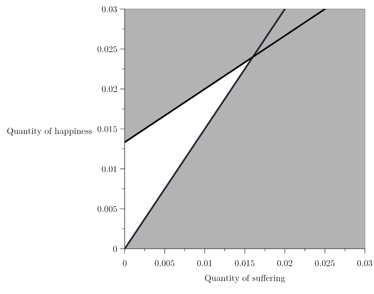
A life \(x_{k}\) is strongly superior to an otherwise identical life \(x_{k + 1}\) with an extra hangnail iff the point picked out by \({s(x}_{k})\) on the horizontal axis and \({h(x}_{k})\) on the vertical axis lies within the unshaded region. This is a welcome result. As we can see, an extra hangnail triggers strong superiority only when added to lives featuring very small quantities of happiness and suffering. The IER View thus gives hangnails their proper axiological due. In blank and nearly blank lives, they can be consequential. In turbulent lives, they pale almost into axiological insignificance.⁠Reflecting this graph in the line \(h = s\) gives the region of lives that can be pushed from bad or strictly neutral to good by an increase of 0.02 in that life’s quantity of happiness. Perhaps this small jump corresponds to a gumdrop’s worth of pleasure. As in figure 7, the region includes only lives featuring very small quantities of happiness and suffering.

I write ‘almost’ because an added hangnail can trigger strong noninferiority, even in turbulent lives. Consider again the case in which \(x_{k}\)⁠’s welfare level is \(\left\langle 9,\ 9 \right\rangle\) and \(x_{k + 1}\)⁠’s welfare level is \(\left\langle 9,\ 9.02 \right\rangle\)⁠. Given \(r_{h} = 0.5\)⁠, \({w(x_{k})}_{r_{h} = 0.5}\)\(= 0.5 \times 9 - 0.5 \times 9\)\(= 0\) and \({w(x_{k + 1})}_{r_{h} = 0.5}\)\(= 0.5 \times 9 - 0.5 \times 9.02\)\(= - 0.01\)⁠. Adding zeroes can never yield a negative number, and vice versa, so any population of lives \(x_{k}\) has greater value than any population of lives \(x_{k + 1}\) relative to \(r_{h} = 0.5\)⁠. That ensures that \(x_{k}\) is strongly noninferior to \(x_{k + 1}\)⁠: any population of lives \(x_{k}\) is not worse than any population of lives \(x_{k + 1}\)⁠.

More generally, an extra hangnail will trigger strong noninferiority whenever at least one of the lives being compared is weakly neutral. In that case, the extra hangnail will push the life’s value from positive to negative relative to some \(r_{h}\)⁠. Relative to that \(r_{h}\)⁠, any population of lives without the hangnail has greater value than any population of lives with the hangnail. Therefore, any population of lives without the hangnail is not worse than any population of lives with the hangnail.

This too is a welcome result. Suppose we must choose between two populations. Each population consists of lives at only one welfare level; one population’s lives are better than the other’s; and at least one population consists of lives that are neither good nor bad. Then it is not worse to choose the population consisting of the better lives, regardless of the populations’ respective sizes.

And importantly, the IER View does not imply strong noninferiority across straightforwardly-better-than-blank lives or strong nonsuperiority across straightforwardly-worse-than-blank lives, as critical-range views do. To see why, consider a life \(y_{k}\) with welfare level \(\left\langle a,\ 0 \right\rangle\) and a life \(y_{k + 1}\) with welfare level \(\left\langle b,\ 0 \right\rangle\)⁠. Suppose that \(a > b > 0\)⁠, so that \(y_{k}\) is better than \(y_{k + 1}\) and both are straightforwardly-better-than-blank. Since both lives feature no suffering whatsoever, \({w(y_{k})}_{r}\) and \({w(y_{k + 1})}_{r}\) are positive relative to each \(r\) in \(R\)⁠. That implies that for any \(r\) in \(R\) and any number \(m\)⁠, there is some number \(n\) such that a population of \(n\) lives \(y_{k + 1}\) has greater value than a population of\(\ m\) lives \(y_{k}\) relative to \(r\). So, for any number \(m\), there is some number \(n\) such that a population of \(n\) lives \(y_{k + 1}\) is better than a population of \(m\) lives \(y_{k}\). The result is that \(y_{k}\) is not strongly noninferior to \(y_{k + 1}\).⁠Indeed, \(y_{k}\) is not even weakly noninferior to \(y_{k + 1}\)⁠. See Chapter 1 of this thesis for the distinction between strong and weak noninferiority. A parallel line of argument proves that no straightforwardly-worse-than-blank life is strongly nonsuperior to any other straightforwardly-worse-than-blank life.

F.4. Less Concerning Greediness

Recall that critical-range views imply Maximal Greediness: for any population of awful lives and any population of wonderful lives, (1) there is some population of straightforwardly-better-than-blank lives such that the population of awful lives is not worse than the population of wonderful lives plus the straightforwardly-better-than-blank lives, or (2) there is some population of straightforwardly-worse-than-blank lives such that the population of wonderful lives is not better than the population of awful lives plus the straightforwardly-worse-than-blank lives. This disjunction follows from critical-range views’ claim that lives at more than one welfare level are contributively weakly neutral and their assumption that any two lives are commensurable. Together, these imply that some straightforwardly-better-than-blank life or some straightforwardly-worse-than-blank life is contributively weakly neutral. And on critical-range views, adding enough contributively weakly neutral lives to a population can make that population incommensurable with any other.

The IER View agrees that lives at more than one welfare level are contributively weakly neutral. On the IER View with \(R = \{ r:0.4 \leq r_{h} \leq 0.6\}\)⁠, for example, lives at \(\left\langle 4,\ 3 \right\rangle\) and \(\left\langle 5,\ 4 \right\rangle\) are both weakly neutral. But, as we have seen, it denies the assumption that any two lives are commensurable. Lives at \(\left\langle 4,\ 3 \right\rangle\) and \(\left\langle 5,\ 4 \right\rangle\) are one such incommensurable pair. As a result, the IER View avoids Maximal Greediness. Blank lives—with welfare level \(\left\langle 0,\ 0 \right\rangle\)—have a value of 0 relative to each \(r\) in \(R\)⁠, and so are contributively strictly neutral. Adding them to a population leaves the new population equally good as the original, so blank lives cannot swallow up goodness or badness.

Straightforwardly-better-than-blank lives, meanwhile—with welfare level \(\left\langle a,\ 0 \right\rangle\)⁠, \(a > 0\)—have positive value relative to each \(r\) in \(R\)⁠, and so are contributively good. Adding them improves a population, so straightforwardly-better-than-blank lives cannot swallow up and neutralize goodness. And mutatis mutandis for straightforwardly-worse-than-blank lives. They cannot swallow up and neutralize badness. Therefore, the IER View implies neither disjunct of Maximal Greediness.

On the IER View, only lives featuring some positive quantity of good can neutralize badness, and only lives featuring some positive quantity of bad can neutralize goodness. This is as it should be.

G. Objections to the Imprecise Exchange Rates View

The above four points constitute the main advantages of the IER View. Below are two objections.

G.1. Some Incommensurability between Good Lives and Weakly Neutral Lives

On the IER View, some good lives are incommensurable with some weakly neutral lives. Take a life \(x\) with welfare level \(\left\langle 1,\ 0 \right\rangle\) and a life \(y\) with welfare level \(\left\langle 8,\ 7 \right\rangle\)⁠. Life \(x\) is good, because \({w(x)}_{r}\) is positive relative to each \(0.4 \leq r_{h} \leq 0.6\)⁠. Life \(y\) is weakly neutral, because \({w(y)}_{r}\) is positive relative to each \(r_{h} > 0.4\dot{6}\) and negative relative to each \(r_{h} < 0.4\dot{6}\)⁠. Yet \(x\) is incommensurable with \(y\)⁠, because \({w(x)}_{r} < {w(y)}_{r}\) relative to each \(r_{h} > 0.5\) and \({w(x)}_{r} > {w(y)}_{r}\) relative to each \(r_{h} < 0.5\)⁠.

Although this consequence might seem odd, we ought to accept it. The reasons are twofold. First, the implication is not unique to the IER View. It is an inevitable consequence of admitting the possibility of lives both weakly neutral and close-to-strictly neutral, as Gustafsson (2020, 96) and Rabinowicz (2020, 86) note. To see why, recall that strictly neutral lives are equally good as the standard and that weakly neutral lives are incommensurable with the standard. These definitions imply that strictly neutral lives are incommensurable with weakly neutral lives. As Raz (1986, 326) notes, a small improvement or detriment to either of two incommensurable objects typically does not remove their incommensurability. Such small tweaks can make a difference only when one of the two objects is almost better than the other. Therefore, if a strictly neutral life is neither almost better nor almost worse than some weakly neutral life, then some good life (slightly better than the strictly neutral life) and some bad life (slightly worse than the strictly neutral life) will also be incommensurable with the weakly neutral life.

Second, incommensurability between some good lives and some weakly neutral lives follows from three claims that we should be reluctant to deny. The first is that a life featuring a positive quantity of good and no bad whatsoever (like a life at welfare level \(\left\langle 1,\ 0 \right\rangle\)⁠) is good. The second is that a turbulent, neutral life (like a life at welfare level \(\left\langle 8,\ 7 \right\rangle\)⁠) can be better than another neutral life (like a life at welfare level \(\left\langle 7,\ 7 \right\rangle\)⁠). The third is that a good life at welfare level \(\left\langle 1,\ 0 \right\rangle\) and a turbulent life at welfare level \(\left\langle 8,\ 7 \right\rangle\) are such that neither is better than the other and a small improvement either way fails to break the deadlock.

G.2. Some Instances of Maximal Repugnance

On the IER View, life \(x\) with welfare level \(\left\langle a,\ 0 \right\rangle\) is good and life \(y\) with welfare level \(\left\langle 0,\ a \right\rangle\) is bad for any \(a > 0\)⁠. That implies that each population of wonderful lives is worse than some population of \(x\)-lives, and each population of awful lives is better than some population of \(y\)-lives. As \(a\) need only be larger than 0, lives \(x\) and \(y\) could be very similar. They could be identical but for \(x\)⁠’s featuring an extra gumdrop and \(y\)⁠’s featuring an extra hangnail. Therefore, the IER View implies Maximal Repugnance. Gustafsson (2020, 96), Broome (2022), and Rabinowicz (2020, 86–87) note that any view admitting the possibility of strictly neutral lives has implications of this kind, and they take it to be a reason to reject such views.

However, I claim that ruling out the IER View on this basis is premature. Note first that implying this instance of Maximal Repugnance seems preferable to the alternative, which is to claim that lives with welfare level \(\left\langle a,\ 0 \right\rangle\) or \(\left\langle 0,\ a \right\rangle\) for some \(a > 0\) are contributively weakly neutral. As we have seen, that claim commits critical-set views to Maximal Greediness.

Note also that the IER View implies Maximal Repugnance only when lives \(x\) and \(y\) are nearly blank. If a life is turbulent, featuring a lot of happiness and suffering, then much more than a few extra gumdrops are required to move that life from bad to good. If we hold a life’s quantity of suffering fixed at 6, for example, then the last contributively bad life has welfare level \(\left\langle 4,\ 6 \right\rangle\) and the first contributively good life has welfare level \(\left\langle 9,\ 6 \right\rangle\)⁠. Once again, the IER View is giving gumdrops and hangnails their proper axiological due. In nearly blank lives, they are significant. In turbulent lives, they fade into the background.

My final point is related. It is common in population axiology to think of lives barely worth living as drab. Parfit (1986, 148) asked us to imagine lives in which the only pleasures are ‘muzak and potatoes.’ But a Muzak and potatoes life can have a welfare level of \(\left\langle a,0 \right\rangle\) only if its protagonist is very different from you and me. We—and everyone else endowed with an ordinary human psychology—would inevitably suffer boredom were we to live such a life, and lives at welfare level \(\left\langle a,0 \right\rangle\) feature no bad whatsoever. So, when we picture lives at \(\left\langle a,\ 0 \right\rangle\)⁠, we should not imagine how we would feel sitting down to another bowl of mashed potatoes. Imagine instead a life of dreamless sleep, topped off with a gumdrop’s worth of pleasure. When I conceive of \(\left\langle a,\ 0 \right\rangle\) lives in this way, the IER View’s implications no longer strike me as so repugnant.

H. Conclusion

The variety of possible critical-set views is dizzying, but each variety has serious drawbacks. On critical-level views, two extra hangnails can mark the difference between a good life and a bad life, even when the lives in question are long and turbulent. That means that a population of just a single life without the hangnails is better than any population of lives with them. It also means that each population of wonderful lives is worse than some population of lives without the hangnails, while each population of awful lives is better than some population of lives with them. On critical-range views, meanwhile, each population of wonderful lives and each population of awful lives is such that adding enough lives featuring only good and neutral components to the former makes it no better than the latter, or adding enough lives featuring only bad and neutral components to the latter makes it no worse than the former. What is more, some discontinuity in contributive value must occur in a counterintuitive place, so that a population of just a single life featuring only dreamless sleep and some duration of happiness is not worse than any population of lives identical but for a slightly shorter duration of happiness, or a population of just a single life featuring only dreamless sleep and some duration of suffering is not better than any population of lives identical but for a slightly shorter duration of suffering. Some varieties of critical-set view are sadistic, and no variety can account for the incommensurability between lives and between same-size populations without extra theoretical resources.

The IER View comes equipped with the required theoretical resources. It diagnoses as the source of incommensurability the fact that some trade-offs are neither worth making nor worth not making and a small improvement fails to break the deadlock. The resulting incommensurability between lives allows us to claim both that blank lives are strictly neutral and that a wide range of turbulent lives are weakly neutral, so that the IER View captures the advantages of both critical-level and critical-range views and charts the narrow course between Maximal Greediness and the most concerning instances of Maximal Repugnance. Making the size of the contributively neutral range depend on a life’s quantity of goods and bads has another nice consequence: it gives gumdrops and hangnails their proper axiological due. When a life is nearly blank, one fewer gumdrop and one extra hangnail can take it from good to bad. When a life is turbulent, gumdrops and hangnails pale almost into axiological insignificance. And because the IER View determines a life’s categories of personal and contributive value in the same way, it escapes all forms of sadism.

In sum, the IER View is a worthy successor to critical-set views. It retains much of their appeal, while avoiding many of their pitfalls.⁠I thank Hilary Greaves, Teruji Thomas, Tomi Francis, Kacper Kowalczyk, Alice van’t Hoff, Todd Karhu, Nikhil Venkatesh, Jessica Fischer, Aidan Penn, Michal Masny, Farbod Akhlaghi, and two anonymous reviewers for the Journal of Ethics and Social Philosophy for helpful comments and discussion. This chapter has been published as Thornley (2022).

8. References

Arrhenius, Gustaf. 2000a. ‘An Impossibility Theorem for Welfarist Axiologies’. Economics & Philosophy 16 (2): 247–66.

———. 2000b. ‘Future Generations: A Challenge for Moral Theory’. PhD Thesis, Uppsala University.

Arrhenius, Gustaf, and Wlodek Rabinowicz. 2015a. ‘The Value of Existence’. In The Oxford Handbook of Value Theory, edited by Iwao Hirose and Jonas Olson, 424–44. New York: Oxford University Press.

———. 2015b. ‘Value Superiority’. In The Oxford Handbook of Value Theory, edited by Iwao Hirose and Jonas Olson, 225–48. New York: Oxford University Press.

Blackorby, Charles, Walter Bossert, and David Donaldson. 1996. ‘Quasi-Orderings and Population Ethics’. Social Choice and Welfare 13 (2): 129–50. https://doi.org/10.1007/BF00183348.

———. 2005. Population Issues in Social Choice Theory, Welfare Economics, and Ethics. Cambridge: Cambridge University Press.

Bossert, Walter. 2022. ‘Anonymous Welfarism, Critical-Level Principles, and the Repugnant and Sadistic Conclusions’. In The Oxford Handbook of Population Ethics, edited by Gustaf Arrhenius, Krister Bykvist, Tim Campbell, and Elizabeth Finneron-Burns. Oxford: Oxford University Press.

Broome, John. 2004. Weighing Lives. Oxford: Oxford University Press.

———. 2022. ‘Loosening the Betterness Ordering of Lives: A Response to Rabinowicz’. In The Oxford Handbook of Population Ethics, edited by Gustaf Arrhenius, Krister Bykvist, Tim Campbell, and Elizabeth Finneron-Burns. Oxford: Oxford University Press. http://users.ox.ac.uk/~sfop0060/pdf/Loosening%20the%20betterness%20ordering%20of%20lives.pdf.

Bykvist, Krister. 2007. ‘The Good, the Bad and the Ethically Neutral’. Economics & Philosophy 23 (1): 97–105.

Carlson, Erik. 1998. ‘Mere Addition and Two Trilemmas of Population Ethics’. Economics & Philosophy 14 (2): 283–306.

Chang, Ruth. 2002. ‘The Possibility of Parity’. Ethics 112 (4): 659–88.

De Sousa, Ronald B. 1974. ‘The Good and the True’. Mind 83 (332): 534–51.

Frick, Johann. 2017. ‘On the Survival of Humanity’. Canadian Journal of Philosophy 47 (2–3): 344–67.

Gustafsson, Johan E. 2020. ‘Population Axiology and the Possibility of a Fourth Category of Absolute Value’. Economics & Philosophy 36 (1): 81–110.

Hudson, James L. 1987. ‘The Diminishing Marginal Value of Happy People’. Philosophical Studies 51 (1): 123–37.

Huemer, Michael. 2008. ‘In Defence of Repugnance’. Mind 117 (468): 899–933.

Meacham, Christopher J. G. 2012. ‘Person-Affecting Views and Saturating Counterpart Relations’. Philosophical Studies 158 (2): 257–87.

Nebel, Jacob M. 2021. ‘Totalism without Repugnance’. In Ethics and Existence: The Legacy of Derek Parfit, edited by Jeff McMahan, Tim Campbell, James Goodrich, and Ketan Ramakrishnan. Oxford: Oxford University Press. https://philpapers.org/archive/NEBTWR.pdf.

Parfit, Derek. 1984. Reasons and Persons. Oxford: Clarendon Press.

———. 1986. ‘Overpopulation and the Quality of Life’. In Applied Ethics, edited by Peter Singer, 145–64. Oxford: Oxford University Press.

Qizilbash, Mozaffar. 2007. ‘The Mere Addition Paradox, Parity and Vagueness’. Philosophy and Phenomenological Research 75 (1): 129–51.

———. 2018. ‘On Parity and the Intuition of Neutrality’. Economics & Philosophy 34 (1): 87–108.

Rabinowicz, Wlodek. 2009. ‘Broome and the Intuition of Neutrality’. Philosophical Issues 19 (1): 389–411.

———. 2020. ‘Getting Personal: The Intuition of Neutrality Reinterpreted’. In Studies on Climate Ethics and Future Generations, Vol. 2, edited by Paul Bowman and Katharina Berndt Rasmussen. Working Paper Series. Stockholm: Institute for Futures Studies. https://www.iffs.se/en/publications/working-papers/studies-on-climate-ethics-and-future-generations-vol-2/.

Raz, Joseph. 1986. The Morality of Freedom. Oxford: Oxford University Press.

Tännsjö, Torbjörn. 2002. ‘Why We Ought to Accept the Repugnant Conclusion’. Utilitas 14 (3): 339–59.

Thornley, Elliott. 2022. ‘Critical Levels, Critical Ranges, and Imprecise Exchange Rates in Population Axiology’. Journal of Ethics and Social Philosophy 22 (3): 382–414.

Chapter 4: Critical-Set Views, Biographical Identity, and the Long Term

Abstract: Critical-set views avoid the Repugnant Conclusion by subtracting some constant from the welfare score of each life in a population. These views are thus sensitive to facts about biographical identity: identity between lives. In this chapter, I argue that questions of biographical identity give us reason to reject critical-set views and embrace the total view. I end with a practical implication. If we shift our credences towards the total view, we should also shift our efforts towards ensuring that humanity survives for the long term.

I. Introduction

Although Tutankhamun has been dead for over three millennia, we have some ideas about his life. He was slight-of-build and may have walked with a cane, the unfortunate result of a curved spine. He came to the Egyptian throne at the age of nine and died about a decade later. Once thought to have been murdered, scholars now believe that his death was accidental. It was perhaps the consequence of a chariot crash (Booth 2007).

Suppose that someday we come to know much more about the life of King Tut. Suppose that Mina — some future scientist — has access to Tut’s DNA, along with information about his memories, desires, and other psychological features. And suppose that Mina creates a duplicate of Tut — Tut* — to these specifications. As this duplicate hobbles around the lab, Mina might wonder: has Tut’s life resumed? Or has a new life begun?

Some will find this question interesting. Others will not, thinking it instead empty or merely verbal. But even these others may find their interest roused by a question of a more practical flavour. Rewind, and suppose that Mina has two options. She can create Tut* who (she knows for sure) will live a good life, or she can create Bukayo — an entirely new person — who will live a slightly better life. Whoever she creates, other people will be unaffected. Which outcome is better?

On one view in population axiology (and granting an assumption I discuss below), the answer is simple. The total view implies that it is better to create Bukayo, because that will result in greater total welfare. On critical-set views, the answer is not so simple. Their verdicts depend on whether Tut’s life will resume. If Tut’s life will not resume, then it is better to create Bukayo. If Tut’s life will resume, then it is better to create Tut* (on critical-level views) or else the two outcomes are incommensurable (on critical-range views).⁠If you think that the question ‘Will Tut’s life resume?’ is empty — that the answer cannot be discovered but at most stipulated — then I can save you some time. Read the following argument, and then skip straight to Section 6:On critical-set views, the value-relation between the two outcomes depends on whether Tut’s life will resume.‘Will Tut’s life resume?’ is an empty question.Value-relations between outcomes cannot depend on the answer to an empty question.(C) Therefore, critical-set views are false.I have some sympathy for this argument, but my case against critical-set views does not rely on it. From now on, I assume that questions of identity between lives are substantive.

In this chapter, I argue that these questions of identity between lives — questions of biographical identity — spell trouble for critical-set views. I end with a practical implication for those aiming to promote the impartial good. If we shift our credences towards the total view, we should also shift our efforts towards reducing the risk of premature human extinction.⁠In Chapter 5 of this thesis, I argue that questions of personal identity pose similar problems for person-affecting views. Those arguments have a similar practical upshot.

J. Framework

Let a life-episode be an episode of a life: a stretch of a person’s life without any gaps. Your third birthday (for example) is a life-episode, as is your twentieth year, as is the next second, as is your life in its entirety. Let biographical identity be a binary relation that obtains between two life-episodes iff they are episodes of the same life.

A life-episode’s welfare is how good that life-episode is for the person living it. I assume that a life-episode’s welfare can be represented by a real-valued function \(w\)⁠, so that life-episode \(x\) has at least as much welfare as life-episode \(y\) iff \(w(x) \geq w(y)\)⁠. I also assume that welfare is interpersonally comparable, so that we can say whether life-episode \(x\) has at least as much welfare as \(y\) even if \(x\) and \(y\) are lived by different people. And I assume that welfare is measurable on a ratio-scale, so that we can talk meaningfully about the ratios of welfare between life-episodes. Some life-episodes are good for the person living them, others are bad for the person living them, and still others are neutral for the person living them. These life-episodes are assigned positive, negative, and zero welfare scores respectively.⁠In this chapter, I ignore the complication that some lives may be undistinguished or weakly neutral (Gustafsson 2020; Rabinowicz 2022).

A population is a set of lives. On the total view, we sum the welfare scores of the lives in a population to get the value of that population. A population \(X\) is at least as good as a population \(Y\) iff the value of \(X\) is at least as great as the value of \(Y\)⁠.⁠Advocates of the total view include Hudson (1987), Tännsjö (2002), and Huemer (2008). On critical-level views, we first subtract some positive constant from the welfare score of each life in a population and then sum the results to get the value of that population. This positive constant is the critical level. As with the total view, \(X\) is at least as good as \(Y\) iff \(X\)⁠’s value is at least as great as \(Y\)⁠’s.⁠Advocates of critical-level views include Blackorby, Bossert, and Donaldson (2005) and Bossert (2022). On critical-range views, we calculate the value of a population on a range of critical levels. \(X\) is at least as good as \(Y\) iff \(X\)⁠’s value is at least as great as \(Y\)⁠’s on every level in the critical range. If neither \(X\) nor \(Y\) is at least as good as the other, they are incommensurable, on a par, or it is indeterminate which is better.⁠Advocates of critical-range views include Broome (2004), who interprets the critical range as a range of indeterminacy, along with Qizilbash (2007; 2018) and Rabinowicz (2009), who each interpret the critical range as a range of parity. I adopt the language of incommensurability in this chapter, but my discussion can be translated into other terms without significant change to its import. Following Chapter 3 of this thesis, I use the term ‘critical-set views’ to refer to that class of views comprising both critical-level and critical-range views.

Here is an example to illustrate the difference between the total view, critical-level views, and critical-range views. Suppose that we can bring about either population \(A\) or population \(B\)⁠, represented by the following sets of welfare scores:

\[A = \left\{ 5 \right\}\](76)

\[B = \{ 2,\ 2,\ 2\}\](77)

On the total view, the value of \(A\) is \(5\) and the value of \(B\) is \(2 + 2 + 2 = 6\)⁠, so \(B\) is better than \(A\)⁠. On a critical-level view with a critical level of 4, the value of \(A\) is \((5 - 4) = 1\) and the value of \(B\) is \((2 - 4) + (2 - 4) + (2 - 4) = - 6\)⁠, so \(A\) is better than \(B\)⁠. On a critical-range view with a critical range running from \(0\) to \(4\)⁠, \(A\) and \(B\) are incommensurable, because \(A\) has greater value on a critical level of \(4\) and \(B\) has greater value on a critical level of \(0\)⁠. For concreteness, I discuss these critical-level and critical-range views below. Everything I write applies — mutatis mutandis — to views with critical levels and ranges occurring elsewhere. I also use the term discount constant to refer to the maximum amount by which a life’s welfare score is discounted in calculating the value of a population. On our example critical-level and critical-range views, the discount constant is \(4\)⁠.

That is all the set-up required for this chapter. Onto the objections.

K. The Drop

Suppose that there exists a machine called the LifeTransformer. Stored on this machine is a digital file, containing all the information needed to create an entirely new person: Leah. At setting \(0\) on the LifeTransformer, nothing happens. Emile walks into the machine and then right back out again, entirely unchanged. At setting \(1\)⁠, a small cluster of cells in Emile’s brain and body are replaced with Leah’s.⁠Or, rather, replaced with a small cluster of cells that would match a small cluster of cells in Leah’s brain, if Leah existed. I leave further qualifications of this kind implicit. As a consequence, the person who walks out — call them Emile* — shares some psychological features with Leah. Perhaps Emile* has a few of Leah’s beliefs and intentions. At higher settings, larger clusters of Emile’s cells are replaced with Leah’s, and Emile* shares more psychological features with Leah. At setting \(1000\)⁠, Emile’s entire brain and body is replaced with Leah’s, and Emile* is exactly like Leah in psychological respects.⁠This case is a cosmetic variation on Parfit’s Combined Spectrum (1984, 236–37).

Now consider the following three outcomes:

Decent: Emile does not enter the LifeTransformer. He lives a life with a welfare score of \(6\)⁠.

Great: Emile does not enter the LifeTransformer. He lives a life with a welfare score of \(8\)⁠.

Composite: Emile lives a life-episode with a welfare score of \(5\)⁠. He then enters the LifeTransformer at some setting. Emile* then lives a life-episode with a welfare score of \(4\)⁠.

Here is a diagram to illustrate:

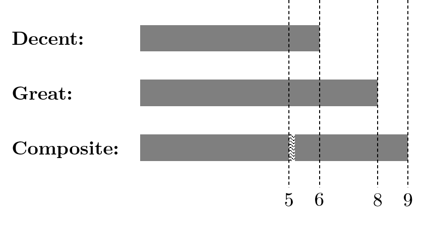
Suppose — for now — that individual welfare is additively separable over life-episodes: that is to say, for all life-episodes \(x\) and \(y\) with welfare scores \(w(x)\) and \(w(y)\) respectively, the life-episode composed of \(x\) and \(y\) has welfare score \(w(x) + w(y)\)⁠.⁠This is the ‘assumption I discuss below’ mentioned in the introduction. Consider two questions:

1. Is Composite better than Great?

2. Is Composite better than Decent?

On the total view, the answers are simple. Composite is better than Great and better than Decent. That is because (ignoring all unaffected lives), the value of Decent is \(6\)⁠, the value of Great is \(8\)⁠, and the value of Composite is \(9\)⁠. On our example critical-set views, the answers are not so simple. They depend on whether Emile and Emile* live the same life.

Consider first our critical-level view, with a critical level of 4. If Emile and Emile* live the same life, the value of Decent is \((6 - 4) = 2\)⁠, the value of Great is \((8 - 4) = 4\)⁠, and the value of Composite is \((9 - 4) = 5\)⁠. Therefore, if Emile and Emile* live the same life, Composite is better than Great.

If Emile and Emile* live different lives, however, the value of Decent is \((6 - 4) = 2\)⁠, the value of Great is \((8 - 4) = 4\)⁠, and the value of Composite is \((5 - 4) + (4 - 4) = 1\)⁠. The value of Composite has decreased, because we now subtract the discount constant \(4\) from two separate welfare scores: Emile’s and Emile*’s. Therefore, if Emile and Emile* live different lives, Composite is worse than Decent.

Clearly, when Emile enters the LifeTransformer at setting \(0\)⁠, he and Emile* live the same life. Equally clearly, when Emile enters the LifeTransformer at setting \(1000\)⁠, he and Emile* live different lives. Therefore, if biographical identity is all-or-nothing, there must be some setting \(k\) such that at \(k\) Emile and Emile* live the same life and at \(k + 1\) Emile and Emile* live different lives.⁠One might deny the antecedent of this conditional: a point which I address below. Our critical-level view then implies an implausibly large drop in the value of Composite as we move from \(k\) to \(k + 1\)⁠. Composite goes from better than Great to worse than Decent, despite the fact that the move from \(k\) to \(k + 1\) involves replacing just a few more of Emile’s cells and psychological features with Leah’s. ⁠This might be considered an example of what Pummer calls hypersensitivity: ‘when a slight difference in one sort of property makes a radical difference in another sort of property.’ (Pummer 2021, 510).

We get a similar drop on critical-range views. Recall that on our example critical-range view we calculate the value of each population on a range of critical levels running from \(0\) to \(4\)⁠. If Emile and Emile* live the same life, the values of Decent, Great, and Composite on a critical level of \(0\) are \(6\)⁠, \(8\)⁠, and \(9\) respectively, while their values on a critical level of \(4\) are \(2\)⁠, \(4\)⁠, and \(5\) respectively. Since the value of each population decreases linearly as the critical level increases, these values at the critical range’s endpoints imply that Composite has greater value than Great on each level in the critical range. Therefore, if Emile and Emile* live the same life, Composite is better than Great.

If Emile and Emile* live different lives, however, the values of Decent, Great, and Composite on a critical level of \(0\) are \(6\)⁠, \(8\)⁠, and \(9\) respectively, and their values on a critical level of 4 are \(2\)⁠, \(4\)⁠, and \(1\) respectively. The value of Composite on a critical level of \(4\) has decreased, because we now subtract the discount constant \(4\) from two separate welfare scores: Emile’s and Emile*’s. Thus, neither Composite nor Decent has at least as much value as the other on each level in the critical range. Composite has greater value on a critical level of \(0\) and Decent has greater value on a critical level of \(4\)⁠. Therefore, if Emile and Emile* live different lives, Composite is incommensurable with Decent.

If biographical identity is all-or-nothing, our critical-range view implies that there is some setting \(k\) such that Composite is better than Great at \(k\) and incommensurable with Decent at \(k + 1\)⁠. This change in evaluative verdicts is not as stark as the change on our critical-level view, but the drop in Composite’s value still seems implausibly sharp. Many changes to Emile’s cells and psychological features make no difference, but one tiny change pushes Composite from better than Great to no better than Decent.

I assumed above that individual welfare is additively separable over life-episodes. That assumption allowed me to infer that, since Emile and Emile*’s welfare scores are \(5\) and \(4\) respectively when they live different lives, their combined welfare score is \(5 + 4 = 9\) when they live the same life. But additive separability over life-episodes is controversial (Broome 2004, 106–9). Many philosophers believe that a life’s welfare score can be greater or lesser than the sum of its parts (see, for example, Dorsey 2015 and references therein). So, it is worth noting that the drop remains a problem when we cease to assume additive separability.

Suppose first that Emile’s and Emile*’s welfare score when they live the same life is greater than \(9\)⁠. In that case, there is still a drop. At \(k\)⁠, Composite is better than Great. At \(k + 1\)⁠, Composite is worse than Decent (on our critical-level view) or else Composite is incommensurable with Decent (on our critical-range view).

So, suppose instead that Emile’s and Emile*’s welfare score when they live the same life is less than \(9\)⁠. In that case, so long as Emile’s and Emile*’s combined welfare score is not exactly equal to \(5\)⁠, there will still be some discontinuity in the value of populations as we ascend the settings on the LifeTransformer. That is because, on our critical-level view, the value of Composite when Emile and Emile* live different lives is \((5 - 4) + (4 - 4) = 1\)⁠. To avoid any discontinuity whatsoever, the value of Composite when they live the same life must also equal \(1\)⁠. Since we subtract the discount constant \(4\) just once when Emile and Emile* live the same life, their combined welfare score must be \(5\)⁠.

More generally, to avoid all discontinuities in LifeTransformer cases on our critical-level view, the longevity penalty (as I will call it) must always equal \(4\)⁠. That is to say, whenever a life-episode \(y\) is appended to a life-episode \(x\)⁠, the welfare score of the combined life-episode must equal \(w(x) + w(y) - 4\)⁠. Then the value of a population would remain the same when life-episodes \(x\) and \(y\) came to belong to different lives, because the application of the extra discount constant would be cancelled out by the loss of the longevity penalty. But then, since even a single moment of a life is a life-episode, our critical-level view must claim that we incur a longevity penalty of \(4\) with each new moment. If the next moment of your life would have a welfare score of less than \(4\) if lived on its own, it would be better for you to die now rather than live it. That seems implausible.

Critical-range views, meanwhile, cannot avoid all discontinuities by denying additive separability. Even if Emile and Emile*’s combined welfare score is exactly equal to 5, there will still be a discontinuity. It will just be in the opposite direction: a jump rather than a drop. On a critical level of \(0\)⁠, the value of Composite when Emile and Emile* live the same life will be \(5\)⁠, while the value of Composite when they live a different life will be \(9\)⁠. Therefore, Composite is worse than Decent at \(k\) and incommensurable with Great at \(k + 1\)⁠.

A more promising way to soften these discontinuities is to move the critical level towards 0 in the case of critical-level views, and to move one or both of the endpoints of the critical range towards \(0\) in the case of critical-range views. If, for example, we lower the critical level from \(4\) to \(3\)⁠, any discontinuity will be smaller. But note two points. First, the closer the critical level and critical range are to \(0\)⁠, the more critical-level and critical-range views behave like the total view. Second, even a small discontinuity seems implausible. The difference between Emile* at \(k\) and Emile* at \(k + 1\) might be no more than a few cells and faint memories: the kind of change that you and I undergo every minute. It is hard to believe that a population featuring Emile* at \(k + 1\) is significantly worse than a population featuring Emile* at \(k\)⁠. To avoid discontinuities entirely, we must have a single critical level at \(0\)⁠, and then the view renders all of the same verdicts as the total view.

A more radical way for advocates of critical-set views to avoid discontinuities is to deny another assumption that I made above. Besides assuming that individual welfare is additively separable over life-episodes, I also assumed that biographical identity is all-or-nothing: that there is some setting \(k\) on the LifeTransformer such that at \(k\) Emile and Emile* live the same life and at \(k + 1\) they live different lives. That led me to assume that the application of the discount constant is also all-or-nothing: that at \(k\) Emile*’s welfare score is discounted by \(0\) and at \(k + 1\) it is discounted by \(4\)⁠. But advocates of critical-set views can deny this last assumption. They can claim instead that the discount to Emile*’s welfare score increases in small increments as we ratchet up the settings on the LifeTransformer. Perhaps at setting \(1\)⁠, Emile*’s welfare score is discounted by 0.004, at setting \(2\)⁠, it is discounted by 0.008, and so on. That would allow critical-set views to avoid any discontinuities. As we ramp up the settings, there will come a point at which Great is better than Composite and Composite is better than Decent on critical-level views, and a point at which Great is incommensurable with Composite and Composite is better than Decent on critical-range views.

This discount-by-degrees — as I will call it — could be justified by claiming that biographical identity is sometimes indeterminate and that this indeterminacy admits of degrees.⁠Lewis (1976) makes these claims about personal identity. A discount-by-degrees could also be justified by claiming that the size of the discount constant depends not on biographical identity but on some relation more commonly thought to come in degrees, such as psychological or physical connectedness.⁠Parfit (1984, 313) makes this claim of prudential decisions: the degree to which we can rationally discount future welfare depends on psychological connectedness. Whichever way the move is justified, however, critical-set views will face an objection from Egyptology.

L. Egyptology

The total view and critical-set views satisfy Separability over Lives: whether an outcome \(A\) is at least as good as an outcome \(B\) depends only on the existence and welfare of lives affected by the choice between \(A\) and \(B\)⁠.⁠Blackorby, Bossert and Donaldson (2005, 127) call this condition Existence Independence. Other views in population axiology — like the average view, variable value views, and rank-discounted views — do not satisfy Separability over Lives: whether \(A\) is at least as good as \(B\) can depend on the existence and welfare of lives unaffected by the choice.⁠See Thomas (2022) and Tarsney and Thomas (2020) for discussion. On these latter views, we may have to do research in Egyptology — figuring out how numerous and well-off the ancient Egyptians were — to determine which of the outcomes available to us is best. That requirement seems implausible, and many take it as a reason to reject such views.⁠See McMahan (1981, 115) for the original point and Parfit (1984, 420) for the ancient Egyptians example.

It is commonly thought that critical-set views — being separable over lives — do not require research in Egyptology.⁠See, for example, Wilkinson (2022, 467). But that is not true. At least, it is not true so long as critical-set views are paired with what I call a non-fire account of biographical identity. I explain the distinction between fire and non-fire accounts below. For now, it suffices to say that, on non-fire accounts, life-episodes need not be spatiotemporally continuous to be part of the same life. Critical-set views paired with non-fire accounts require Egyptology whether they feature an all-or-nothing discount constant or a discount-by-degrees.

To see how, recall the case of Mina and Tutankhamun. Assume for now that individual welfare is additively separable over life-episodes, and suppose for concreteness that Tut’s ancient Egyptian life-episode has a welfare score of 10, Tut*’s life-episode would have a welfare score of 9, and Bukayo’s life-episode would have a welfare score of 10. On our critical-level view, creating Tut* is better than creating Bukayo iff the discount \(d\) applied to Tut*’s welfare score is less than 3, and creating Bukayo is better than creating Tut* iff \(d\) is greater than 3.⁠Ignoring all unaffected lives, and supposing that Tut’s and Bukayo’s lives are entirely new and hence fully discounted, the value of creating Bukayo is \((10 - 4) + (10 - 4) = 12\)⁠, while the value of creating Tut* is \((10 - 4) + (9 - d)\)⁠. If \(d < 3\)⁠, creating Tut* has more value. If \(d > 3\)⁠, creating Bukayo has more value. On our critical-range view, creating Tut* is incommensurable with creating Bukayo iff \(d\) is less than 3, and creating Bukayo is better than creating Tut* iff \(d\) is greater than or equal to 3.⁠Creating Bukayo is never worse than creating Tut*, because creating Bukayo has greater value on a critical level of \(0\)⁠: the value of creating Bukayo is \((10 - 0) + (10 - 0) = 20\) and the value of creating Tut* is \((10 - 0) + (9 - 0) = 19\)⁠. Creating Tut* is incommensurable with creating Bukayo iff \((10 - 4)\)\(+ (9 - d)\)\(> (10 - 4)\)\(+ (10 - 4)\)⁠, where \(d\) is the maximum discount applied to Tut*’s welfare. That is, iff \(d < 3\)⁠. Therefore, on our critical-set views, which outcome is best depends on the size of the discount applied to Tut*’s welfare score. And that in turn depends on whether Tut and Tut* live the same life, or else on the extent to which Tut* resembles Tut in certain respects. Thus, on our critical-set views, Mina may need to read up on Tut’s life and figure out how closely his memories, desires, and other psychological features would be matched by Tut*’s in order to determine which of the outcomes available to her is best. That requirement seems implausible.

As above, I have thus far assumed that individual welfare is additively separable over life-episodes. But, again as above, denying additive separability is an unappealing escape-route. We can avoid the need for Egyptology on critical-level views only if the longevity penalty is \(4 - d\)⁠. Then in cases where Tut and Tut* are similar, the discount \(d\) is low and the longevity penalty is high, while in cases where Tut and Tut* are dissimilar, the discount \(d\) is high and the longevity penalty is low. In each case, the value of the population resulting from Mina’s creating Tut* remains the same, so Mina can know the value of creating Tut* without knowing how closely Tut* resembles Tut. But, as before, this view is implausible with respect to welfare. It implies that, with each passing undiscounted moment of your life, you incur a longevity penalty of 4. If your next moment is undiscounted and would have a welfare score of less than 4 were it lived alone, it would be better for you to die now rather than live it.

Critical-range views, meanwhile, cannot avoid Egyptology by denying additive separability. If a longevity penalty cancels out the effect of a discount from some level in the critical range, it will fail to cancel out a discount from some other level. Thus, the value of Mina’s creating Tut* on at least one level in the critical range — and hence whether it is better to create Tut* than some other life — will depend on how closely Tut* resembles Tut.

Rather than avoid Egyptology, advocates of critical-set views might instead accept it. They might agree that the value-relations pertinent to Mina’s choice depend on the extent to which Tut* resembles Tut. If Tut* bears little resemblance to Tut, creating Tut* is more like creating a new life and Tut*’s welfare should be heavily discounted. If Tut* bears a strong resemblance to Tut, then creating Tut* is more like bringing Tut back from the dead and Tut*’s welfare should be discounted little if at all. Bringing people back from the dead is better than creating new lives.

Even with this rationale, however, the need for Egyptology still seems like a blow. It seems implausible to claim that which of Mina’s available outcomes is best could depend on — say — whether an ancient Egyptian Pharaoh liked the taste of honey. More implausible still is the following implication: which outcome is best could depend on the resemblance between Tut and Tut* even if Tut’s life was (and Tut*’s life would be) not particularly rich or varied: even if, for example, Tut’s life was (and Tut*’s life would be) no more than an unbroken period of mild and uniform pleasure.⁠This proviso rules out cases in which Tut* would complete some project of Tut’s or satisfy some of Tut’s desires: cases in which it might seem more plausible that the value of the available outcomes depends on the resemblance between Tut and Tut*. What is more, I expect these implications to seem especially worrying to advocates of critical-set views. After all, one of the major attractions of these views was that they seemed to avoid the need for Egyptology (Wilkinson 2022, 467).

What seems to me a better response is to pair critical-set views with a fire account of biographical identity. On fire accounts, lives are like fires.⁠Analogies along these lines are old. See Seneca (2004, Letter LIV, 104-5): Wouldn't you say that anyone who took the view that a lamp was worse off when it was put out than it was before it was lit was an utter idiot? We, too, are lit and put out. We suffer somewhat in the intervening period, but at either end of it there is deep tranquillity. See also the Aggi-Vacchagotta Sutta (Majjhima Nikāya 72), in which the Buddha compares asking where an enlightened person goes after death to asking where a fire goes after it is blown out. Their identity requires both spatial and temporal continuity. Putting out a fire and then lighting another in the same place does not bring back the same fire, no matter how close the resemblance. The gap in temporal continuity means that the old fire is gone forever. Similarly for spatial continuity. A fire lit in a different place at the same instant some fire is put out is not the same fire, no matter how similar they are in other respects. On fire accounts, lives are the same. To die for an instant is to die forever.

For an example of a fire account, consider a version of McMahan’s Embodied Mind account of personal identity (2002, chap. 1.5), amended so that it refers to lives rather than persons. On this account, biographical identity consists in the continued existence and functioning of enough of the same brain to support the capacity for consciousness.

Advocates of critical-set views can use fire accounts to address my Drop and Egyptology objections. They can avoid the drop by claiming that the discount applied to Emile*’s welfare score increases in small increments as we ramp up the settings on the LifeTransformer, or else they can justify the drop by appealing to their criterion of biographical identity. If they adopt an Embodied Mind account, for example, they can claim that the drop should come as no surprise: despite the small physical and psychological differences between Emile* at \(k\) and Emile* at \(k + 1\)⁠, passing through the LifeTransformer at \(k\) preserves Emile’s capacity for consciousness and passing through at \(k + 1\) does not. Fire accounts also imply that Mina need not do research in Egyptology. Since there is no spatiotemporal continuity between Tut and Tut*, she can be sure that creating Tut* means creating a new life. Which of the available outcomes is best will not depend on how closely Tut* resembles Tut.

However, trouble remains. Advocates of critical-set views may be surprised to find themselves driven towards such a narrow class of views about biographical identity. They may also be reluctant to accept some of fire accounts’ implications. Consider, for example, Parfit’s Teletransporter (1984, 199), which vaporises your brain and body and then creates a perfect replica out of new matter. Since the Teletransporter does not preserve spatiotemporal continuity between you and your replica, fire accounts imply that your life ends when you enter. And a variation on Parfit’s Teletransporter throws up some unsavoury ethical implications. First imagine a long, wonderful life. Then suppose that some event like this life occurs, except that the brain and body at its centre are momentarily and frequently blinked out of and then back into existence. Call this event a wonderful-but-blinking life-series. Since fire accounts imply that each blink causes the end of one life and the beginning of another, critical-set views paired with a fire account imply that the welfare scores of each of these short lives is discounted. If the blinks occur frequently enough, the value of each wonderful-but-blinking life-series on a positive critical level will be arbitrarily low. That means that critical-level views paired with a fire account imply the Blinking Sadistic Conclusion:

For any population of awful lives, there is some population of wonderful-but-blinking life-series such that the blinking population is worse than the awful population.

Critical-range views, meanwhile, imply the Weak Blinking Sadistic Conclusion:

For any population of awful lives, there is some population of wonderful-but-blinking life-series such that the blinking population is not better than the awful population.⁠For the original Sadistic Conclusion, see Arrhenius (2000, 256). For the Weak Sadistic Conclusion, see Gustafsson (2020, 86).

Both conclusions seem tough to accept, since the blinking population is exactly like a population of wonderful lives except for the blinks.

Advocates of critical-set views might react by holding on to fire accounts and accepting a Blinking Sadistic Conclusion, or else by rejecting fire accounts and accepting the need for Egyptology. Neither option strikes me as appealing, and both options lead to trouble in cases of fission.

M. Fission

Suppose that Asiya’s brain is divided in two, and each half is implanted into an exact replica of her body. Each of the resulting people — call them Lefty and Righty — share all of Asiya’s psychological features. Both Lefty and Righty are also phenomenally, physically, and functionally continuous with pre-fission Asiya. That is to say, Asiya’s stream of (and capacity for) consciousness divides and flows uninterrupted into the streams of (and capacities for) consciousness of Lefty and Righty.⁠This is a cosmetic variation on Parfit’s My Division (1984, 254–55).

In this case, which — if any — of Lefty’s and Righty’s welfare scores is discounted? Here are six possible answers.

1. Both Lefty’s and Righty’s welfare scores are discounted.

2. Lefty’s welfare score is discounted.

3. Righty’s welfare score is discounted.

4. One of Lefty’s and Righty’s welfare scores is discounted, but it is indeterminate which.

5. Each of Lefty’s and Righty’s welfare scores is ‘half-discounted’.

6. Neither Lefty’s nor Righty’s welfare scores is discounted.

I believe that only (6) is viable. Each of (1)-(5) implies some especially implausible Sadistic Conclusion. To see how, suppose that Asiya splits into Lefty and Righty. Each of Lefty and Righty then live a life-episode with a welfare score of 1, before themselves splitting in two. Each of their descendants also lives a life-episode with a welfare score of 1 before splitting in two, and so on. Call this a good-but-splitting life-tree. On answers (1)-(5) and a critical level of 4, each split reduces the population’s value: each of the two splittees lives a life-episode with a welfare score of 1, but the welfare discount is at least 4.⁠On (1), each of Lefty’s and Righty’s welfare scores is discounted by 4, for a total discount of 8. On (2), (3), and (4), one of Lefty’s and Righty’s welfare scores is discounted by 4, for a total discount of 4. On (5), each of Lefty’s and Righty’s welfare scores is discounted by 2, for a total discount of 4. That means that our critical-level view paired with (1)-(5) implies the Splitting Sadistic Conclusion:

For any population of awful lives, there is a population of good-but-splitting life-trees that is worse.

Our critical-range view paired with (1)-(5), meanwhile, implies the Weak Splitting Sadistic Conclusion:

For any population of awful lives, there is a population of good-but-splitting life-trees that is not better.

These Splitting Sadistic Conclusions are more troubling than the originals, since each splittee can be psychologically, phenomenally, physically, and functionally continuous with all of their ancestors and descendants. Their lives need not be lives of ‘muzak and potatoes’ either (Parfit 1986, 148). In fact, each splittee’s life-episode can be almost exactly like an episode within a long, wonderful life. The only difference is that this life frequently branches, with each descendant also living a life-episode almost exactly like an episode within a long, wonderful life.

Thus, I take it that advocates of critical-set views will opt for (6): when Asiya splits, neither Lefty’s nor Righty’s welfare score is discounted. That answer allows critical-set views to avoid both forms of Splitting Sadistic Conclusion. The catch is that (6) exposes critical-set views to analogues of all of the problems that afflict the total view, in addition to the classic problems for critical-set views like the original Sadistic and Weak Sadistic Conclusions.⁠For other objections to critical-set views, see Chapter 3 of this thesis.

Consider first the Repugnant Conclusion (Parfit 1984, 388):

For any population of wonderful lives, there is a population of lives barely worth living that is better.

The total view implies the Repugnant Conclusion, while our example critical-set views do not. However, critical-set views paired with (6) do imply the Splitting Repugnant Conclusion:

For any population of wonderful lives, there is a population of life-branches barely worth living that is better.

By ‘life-branch’ I mean the kind of life-episode lived by Lefty and Righty: life-episodes that begin post-fission. To see how critical-set views plus (6) imply the Splitting Repugnant Conclusion, consider a finite but arbitrarily large population of wonderful lives. Call this population \(A\)⁠. Population \(B\) starts out with the same number of lives as \(A\)⁠, but each life immediately splits and the welfare score of each splittee’s life-branch is half of the welfare score of the \(A\)-lives. \(C\) is similar to \(B\)⁠, except that each life immediately splits twice and the welfare score of each splittee’s life-branch is a quarter of the welfare score of the \(A\)-lives. And so on until we reach \(Z\)⁠, in which each \(A\)-life immediately splits many times and each splittee’s life-branch is barely worth living. Perhaps the only pleasures in each such life-branch are muzak and potatoes (Parfit 1986, 148). \(Z^{+}\) is identical to \(Z\) but for a gumdrop’s worth of pleasure added to each life-branch. (6) states that the welfare score of each splittee’s life-branch is undiscounted. Critical-set views then imply that \(Z^{+}\) is better than \(A\)⁠.⁠Why do I render the Splitting Repugnant Conclusion in terms of life-branches rather than lives? Because one might claim that fission preserves biographical identity: when Asiya splits into Lefty and Righty, there remains just one life (Dainton (1992) makes this kind of claim about personal identity: Asiya, Lefty, and Righty are each identical to each other). One might argue for this claim as follows: Asiya’s life-episode is biographically identical to both Lefty’s and Righty’s life-episodes, and identity is transitive, therefore Lefty’s and Righty’s life-episodes are biographically identical. One might also accept what Gustafsson and Kosonen (2021) call the Prudential Total View, on which a life’s welfare score is the sum of the welfare scores of each of its moments (even if some of those moments are lived simultaneously). These claims imply that the lives in \(Z^{+}\) are not barely worth living. Each branch is barely worth living, but each life is wonderful in virtue of its many branches. I take it that advocates of critical-set views will find the Splitting Repugnant Conclusion concerning even if they accept this argument. After all, the \(Z^{+}\) world could be almost exactly like the large-population world in the original Repugnant Conclusion. Both could contain a vast number of human beings subsisting on muzak, potatoes, and a single gumdrop. The only difference would be in origins: the human beings in \(Z^{+}\) would be the product of fission.

More generally, wherever creating new lives presents a problem for the total view, creating new life-branches presents an analogous problem for critical-set views paired with (6). Consider an example. Given a plausible principle about the link between value and reasons, the total view implies that we have reason to create lives barely worth living. Then given a plausible principle about the link between reasons and obligations (and in the absence of any countervailing considerations), the total view implies that we are obliged to create lives barely worth living. That might seem implausible. However, critical-set views paired with (6) have a similarly implausible implication. Given plausible principles about the links between value, reasons, and obligations, critical-set views imply that we are obliged to create life-branches barely worth living.

The upshot is that fission presents a real challenge to critical-set views. If advocates claim that some discount constant applies in fission cases, critical-set views imply some Splitting Sadistic Conclusion. If, on the other hand, advocates claim that no discount constant applies in fission cases, critical-set views face analogues of all of the problems that blight the total view, in addition to the classic problems faced by critical-set views alone.

Thus, I claim, considerations of biographical identity give us reason to reject critical-set views in favour of the total view. Once we begin asking questions about identity between lives, critical-set views run into all kinds of difficulties. Paired with some claims about biographical identity, they entail implausible discontinuities in the value of populations. Paired with other claims, they require research in Egyptology to determine which outcome available to us is best. And no matter what our views about biographical identity, they have troubling consequences in fission cases.

N. Practical Implications

Suppose, then, that we shift some portion of our credence from critical-set views to the total view. This move has practical implications for those of us aiming to promote the impartial good.

To see how, consider an example. You have £\(1\) billion at your disposal. As it stands, you estimate that there is a \(10\%\) chance that humanity goes extinct this century (in which case total future welfare scores will be roughly zero) and a \(90\%\) chance that \(10^{16}\) people exist in the future, with an average welfare score of \(10\) in expectation.⁠\(10^{16}\) is Bostrom’s (2013, 18) conservative estimate of future population size, conditional on avoiding near-term catastrophe. You have two options:

1. Donate to the Nuclear Threat Initiative, and thereby reduce the risk of human extinction this century from \(10\%\) to \(9.99\%\)⁠.⁠The Nuclear Threat Initiative is a non-profit aiming to prevent global catastrophes. See www.nti.org/about for more details.

2. Donate to Emergent Ventures, and thereby increase expected average future welfare scores conditional on survival from \(10\) to \(10.01\)⁠.⁠Emergent Ventures is a grant program aimed at funding ideas for meaningfully improving society. See www.mercatus.org/emergent-ventures for more details.

On the total view, the expected value of donating to the Nuclear Threat Initiative is \((0.099 \times 0)\)\(+ \left( 0.901 \times 10 \times 10^{16} \right)\)\(= 9.01 \times 10^{16}\)⁠, and the expected value of donating to Emergent Ventures is \((0.1 \times 0)\)\(+ \left( 0.9 \times 10.01 \times 10^{16} \right)\)\(= 9.009 \times 10^{16}\)⁠. Therefore, given expected value theory, the total view implies that it is better to donate to the Nuclear Threat Initiative.⁠Expected value theory states that an option \(A\) is at least as good as an option \(B\) iff the expected value of \(A\) is at least as great as the expected value of \(B\)⁠, where the expected value of an option is defined as the probability-weighted average of the values of that option’s possible outcomes.There are many ways to deviate from expected value theory. For instance, theories can recommend that we instead maximise the expectation of some strictly increasing transformation of value, or they can place extra weight on some outcomes (see, e.g., Buchak 2013). These theories require that I tweak my example, but do not affect the general point that I make below.

On our critical-level view, meanwhile, the expected value of donating to the Nuclear Threat Initiative is \((0.099 \times 0)\)\(+ \left( 0.901 \times (10 - 4) \times 10^{16} \right)\)\(= 5.406 \times 10^{16}\)⁠, and the expected value of donating to Emergent Ventures is \((0.1 \times 0)\)\(+ \left( 0.9 \times (10.01 - 4) \times 10^{16} \right)\)\(= 5.409 \times 10^{16}\)⁠. So, given expected value theory, our critical-level view implies that it is better to donate to Emergent Ventures. Since donating to Emergent Ventures has greater value on a critical level of \(4\) and donating to the Nuclear Threat Initiative has greater value on a critical level of \(0\)⁠, our critical-range view implies that the two options are incommensurable.

In this case, then, shifting some portion of our credence from critical-set views to the total view enhances the appeal of donating to the Nuclear Threat Initiative. More generally, placing more stock in the total view increases the relative importance of ensuring humanity’s long-term survival and decreases the relative importance of improving humanity’s prospects conditional on survival.

This effect seems to persist on a Maximise Expected Choiceworthiness (MEC) approach to moral uncertainty (MacAskill, Bykvist, and Ord 2020). According to MEC, in cases of moral uncertainty we are required to maximise expected choiceworthiness, where the expected choiceworthiness of an option is defined as the credence-weighted average of its choiceworthiness on each of the first-order moral theories in which we have credence.⁠At least, this is what we are required to do when all of the theories in which we have credence assign cardinal and intertheoretically-unit-comparable choiceworthiness scores. More complex proposals have been offered for cases where this condition is not met (MacAskill 2016; Tarsney 2019; 2021; MacAskill, Bykvist, and Ord 2020).

Greaves and Ord (2017) prove that — granted certain assumptions⁠The assumptions are as follows: (1) our credence is invested only in complete, acyclic axiologies that assign cardinal choiceworthiness scores; (2) our credence is invested only in axiologies that satisfy a condition of axiological invariance, so that the value of each population does not depend on which population is actual; and (3) the choiceworthiness scores assigned by each of the theories in which we have credence are intertheoretically-unit-comparable (and if a theory’s choiceworthiness scores are normalised in some way, the normalisation does not depend on the base population size).As Greaves and Ord (2017, 141) note, these assumptions are non-trivial restrictions to their analysis. Nevertheless, it seems reasonable to expect that relaxing these assumptions will not alter their headline result. Although the broader analysis will be complex, the basic rationale is simple: on the total view and critical-level views, non-present, non-necessary, and non-actual people matter, and the extent to which they matter increases linearly with their number. — MEC has an interesting implication in cases like the above, where you can affect the expected number of lives that are ever lived. The implication is as follows: if the populations under consideration are sufficiently large in expectation, our effective axiology ­– our ranking of populations under moral uncertainty — matches the axiology of a critical-level view, with a critical level that is the credence-weighted average of the various critical levels in which we have credence.

Greaves and Ord then argue that — granted further assumptions⁠The further assumptions are as follows: (1) our credence is invested only in the total view, critical-level views, and presentist and necessitarian person-affecting views; (2) the intertheoretic-unit-comparisons between these theories are such that they agree on the value of changes to the welfare scores of already existing people; and (3) our credence in the disjunction of the total view and critical-level views is not exceedingly small. As before, these are non-trivial restrictions to Greaves’ and Ord’s analysis. As before, it seems reasonable to expect that relaxing these assumptions will not alter their headline result. — the future population is large enough in expectation to render their result practically significant (2017, 156–59). MEC implies that we residents of the twenty-first century are required to act in accordance with a critical-level view in certain realistic cases, even if our credence in the total view and critical-level views is low. These cases include a case like the above, in which we can reduce the risk of premature human extinction, along with a case in which we can incur some cost in the near future to increase the chance that humanity settles the stars in the far future.

If my arguments from biographical identity are convincing, their effect will be to lower the critical level of our effective axiology. That is because the total view is equivalent to a critical-level view with a critical level of \(0\)⁠. Shifting our credences from proper critical-level views to the total view thus means shifting our credences from positive critical levels to a \(0\) critical level, lowering the credence-weighted average.⁠I am not aware of any philosopher that has non-trivial credence in a critical-level view with a negative critical level. That view implies that we can improve a population by adding bad lives. The practical upshot, as before, is an increase in the relative importance of avoiding premature human extinction and a corresponding decrease in the relative importance of trajectory changes.⁠Note that I have not mentioned critical-range views in the last few paragraphs. These views are excluded from Greaves’ and Ord’s analysis, because they imply that the ‘at least as good as’ relation is incomplete over the set of populations. However, accommodating these views does not seem too difficult. Critical-range views (like the total view and critical-level views) will overpower other population axiologies in various large-population limits, since (like the total view and critical-level views) they imply that non-present, non-necessary, and non-actual people matter, and that the extent to which they matter increases linearly with their number. Our effective axiology in these large-population limits will thus be a critical-range view, with a critical range whose upper (lower) limit is the credence-weighted average of the different upper (lower) limits in which we have credence (and where a single critical level is treated as both the upper and lower limit of a degenerate critical range). In this case, the main effect of my arguments from biographical identity will be to decrease the upper limit of the critical range of our effective axiology. As before, that increases the importance of avoiding premature human extinction, relative to the importance of making trajectory changes.

O. Conclusion

Critical-set views avoid the Repugnant Conclusion by subtracting some constant from the welfare score of each life in a population. These views are thus sensitive to facts about biographical identity, and this sensitivity raises a whole host of problems. If the application of the discount constant is all-or-nothing, critical-set views lead to implausible discontinuities in the value of populations. Severing one synapse and erasing one faint memory can make a population significantly worse. If biographical identity does not require spatiotemporal continuity, then critical-set views require us to become Egyptologists to determine which of some set of outcomes is best. And if biographical identity does require spatiotemporal continuity, then critical-set views imply some Blinking Sadistic Conclusion. We can add some Splitting Sadistic Conclusion to the list of charges if the welfare scores of splittees are discounted. And if the welfare scores of splittees are not discounted, critical-set views imply the Splitting Repugnant Conclusion instead, along with analogues of all the other problems faced by the total view.

So, I argue, we should reject critical-set views in favour of the total view. This move has practical implications for those of us aiming to promote the impartial good. It decreases the relative importance of improving humanity’s future conditional on survival, and increases the relative importance of ensuring that humanity has a future.

8. References

Arrhenius, Gustaf. 2000. ‘An Impossibility Theorem for Welfarist Axiologies’. Economics & Philosophy 16 (2): 247–66.

Blackorby, Charles, Walter Bossert, and David Donaldson. 2005. Population Issues in Social Choice Theory, Welfare Economics, and Ethics. Cambridge: Cambridge University Press.

Booth, Charlotte. 2007. The Boy Behind the Mask: Meeting the Real Tutankhamun. Oxford: Oneworld.

Bossert, Walter. 2022. ‘Anonymous Welfarism, Critical-Level Principles, and the Repugnant and Sadistic Conclusions’. In The Oxford Handbook of Population Ethics, edited by Gustaf Arrhenius, Krister Bykvist, Tim Campbell, and Elizabeth Finneron-Burns. Oxford: Oxford University Press.

Bostrom, Nick. 2013. ‘Existential Risk Prevention as Global Priority’. Global Policy 4 (1): 15–31.

Broome, John. 2004. Weighing Lives. Oxford: Oxford University Press.

Buchak, Lara. 2013. Risk and Rationality. Oxford: Oxford University Press.

Buddha, Gautama. n.d. ‘Aggi-Vacchagotta Sutta’. In Majjhima Nikāya, 72. https://www.dhammatalks.org/suttas/MN/MN72.html.

Dainton, Barry F. 1992. ‘Time and Division’. Ratio 5 (2): 102–28.

Dorsey, Dale. 2015. ‘The Significance of a Life’s Shape’. Ethics 125 (2): 303–30.

Gustafsson, Johan E. 2020. ‘Population Axiology and the Possibility of a Fourth Category of Absolute Value’. Economics & Philosophy 36 (1): 81–110.

Hudson, James L. 1987. ‘The Diminishing Marginal Value of Happy People’. Philosophical Studies 51 (1): 123–37.

Huemer, Michael. 2008. ‘In Defence of Repugnance’. Mind 117 (468): 899–933.

Lewis, David. 1976. ‘Survival and Identity’. In The Identities of Persons, edited by Amelie Oksenberg Rorty, 17–40. University of California Press.

McMahan, Jefferson. 1981. ‘Problems of Population Theory’. Edited by R. I. Sikora and Brian Barry. Ethics 92 (1): 96–127.

———. 2002. The Ethics of Killing: Problems at the Margins of Life. New York: Oxford University Press.

Parfit, Derek. 1984. Reasons and Persons. Oxford: Clarendon Press.

———. 1986. ‘Overpopulation and the Quality of Life’. In Applied Ethics, edited by Peter Singer, 145–64. Oxford: Oxford University Press.

Pummer, Theron. 2021. ‘Sorites on What Matters’. In Ethics and Existence: The Legacy of Derek Parfit, edited by Jeff McMahan, Tim Campbell, James Goodrich, and Ketan Ramakrishnan, 498–523. Oxford: Oxford University Press.

Qizilbash, Mozaffar. 2007. ‘The Mere Addition Paradox, Parity and Vagueness’. Philosophy and Phenomenological Research 75 (1): 129–51.

———. 2018. ‘On Parity and the Intuition of Neutrality’. Economics & Philosophy 34 (1): 87–108.

Rabinowicz, Wlodek. 2009. ‘Broome and the Intuition of Neutrality’. Philosophical Issues 19 (1): 389–411.

———. 2022. ‘Getting Personal: The Intuition of Neutrality Reinterpreted’. In The Oxford Handbook of Population Ethics, edited by Gustaf Arrhenius, Krister Bykvist, Tim Campbell, and Elizabeth Finneron-Burns. Oxford: Oxford University Press. https://www.iffs.se/en/publications/working-papers/studies-on-climate-ethics-and-future-generations-vol-2/.

Seneca, Lucius Annaeus. 2004. Letters from a Stoic. Translated by Robin Campbell. London: Penguin Books.

Tännsjö, Torbjörn. 2002. ‘Why We Ought to Accept the Repugnant Conclusion’. Utilitas 14 (3): 339–59.

Tarsney, Christian J., and Teruji Thomas. 2020. ‘Non-Additive Axiologies in Large Worlds’. https://globalprioritiesinstitute.org/christian-tarsney-and-teruji-thomas-non-additive-axiologies-in-large-worlds/.

Thomas, Teruji. 2022. ‘Separability and Population Ethics’. In The Oxford Handbook of Population Ethics, edited by Gustaf Arrhenius, Krister Bykvist, Tim Campbell, and Elizabeth Finneron-Burns, 271–95. Oxford: Oxford University Press.

Wilkinson, Hayden. 2022. ‘In Defence of Fanaticism’. Ethics 132 (2): 445–77.

Chapter 5: Person-Affecting Views, Personal Identity, and the Long Term

Abstract: On person-affecting views in population ethics, the moral import of a person’s welfare depends on that person’s temporal or modal status (in particular, on whether that person presently exists, actually exists, or will exist regardless of one’s decision). These views typically imply that — all else equal — we’re never required to create extra people, or to act in ways that increase the probability of extra people coming into existence.

In this chapter, I use two of Parfit’s puzzles about personal identity to draw out some implausible consequences of person-affecting views. In cases like Combined Spectrum, such views imply that tiny differences in the physical and psychological connections between persons can engender enormous differences in our moral obligations. And cases like My Division give rise to a dilemma for person-affecting views: either they forfeit their seeming-advantages and face analogues of all of the problems faced by impersonal views like total utilitarianism, or else they turn out to be not so person-affecting after all.

P. Introduction

Suppose that you find yourself with a choice. You can either:

(a) Donate $4500 to the Against Malaria Foundation (AMF).

Or:

(b) Donate $4500 to the Nuclear Threat Initiative (NTI).

You’re confident that donating to AMF would save a child from dying of malaria. You’re also reasonably sure that this child would go on to live an additional 70 years of good life. On the other hand, you estimate that donating to NTI would increase the probability that humanity survives the coming century by about one-in-ten-quadrillion (\(10^{- 16}\)⁠). And you expect that if humanity survives the coming century, the future will contain one-hundred-quadrillion (\(10^{17}\)⁠) good lives, each lasting around 70 years. Where should you send your money?

Here’s a quick argument for NTI. By donating to AMF, you’d cause about 70 additional years of good life to be lived, in expectation. By donating to NTI, you’d cause about 700 additional years of good life to be lived, in expectation. It’s better to add 700 years of good life than it is to add 70 years of good life. Therefore, you should send your money to NTI.

There are many ways to resist this quick argument.⁠Perhaps justice demands that you donate to AMF. Perhaps the child who would benefit from your AMF donation has a right to your help. Perhaps you have agent-relative reasons to favour the child, since they live at the same time as you (see Setiya 2014; Mogensen 2019b for related arguments). Perhaps donating to AMF would cause more years of good life to be lived in expectation, once we consider long-term effects. Perhaps you’re permitted to be risk-averse with respect to the good you do (though see Greaves, MacAskill, and Mogensen, n.d.). Perhaps donating to NTI would be objectionably reckless (or fanatical), since you think it overwhelmingly likely that your donation will make no difference to whether humanity survives or goes extinct (Monton 2019; though see Beckstead and Thomas 2021; Wilkinson 2022). Perhaps you can discount the benefits of donating to NTI, simply because they’d occur further in the future (though see Greaves 2017a). Perhaps you’re so clueless about your donations’ indirect effects that you’re permitted to assign imprecise probabilities to various outcomes, and perhaps these imprecise probabilities in combination with the right decision-rule imply that donating to AMF is permissible (see Greaves 2016; Mogensen 2021 for related arguments). Perhaps the ex ante benefits you bestow on possible people by donating to NTI are so trivial in comparison to the benefits stemming from your AMF donation that you’re never required to donate to NTI, no matter how many people would benefit (Scanlon 1998, 235; Voorhoeve 2014; Cowie and Lawler, n.d.; though see Frick 2015, sec. 8; Mogensen 2019a, 11; Greaves and MacAskill 2021, 28). Perhaps — contra my description — the extra lives that might result from your NTI donation are not good: lives featuring no harms are merely neutral, and lives featuring any harm whatsoever are bad (Fehige 1998; Benatar 2006). Perhaps populations featuring different (numbers of) people are always incommensurable, so that donating to NTI is guaranteed to have an outcome no better than the outcome of donating to AMF (Heyd 1988; Bader 2022). Perhaps your estimate of the NTI donation’s expected value requires a further Bayesian adjustment (Karnofsky 2011). Perhaps donating to AMF is made permissible by the fact that the evidence backing your estimate of the NTI donation’s expected value is comparatively weak. Perhaps the most natural way is to claim that the years of good life that might result from your NTI donation just don’t matter in the same way as the years of good life that would result from your AMF donation. By donating to AMF, you gift 70 more years to a person who actually exists, who will exist regardless of your decision, and who exists right now. The same can’t be said of your donation to NTI. The vast majority of those additional years would accrue far in the future: to people who do not and need never exist.

This is a person-affecting response to the quick argument. On person-affecting views in population ethics, the moral import of a person’s welfare depends on that person’s temporal or modal status. These views typically imply that — all else equal — we’re never required to create extra people, or to act in ways that increase the probability of extra people coming into existence.

Person-affecting views have appealing foundations. They often have their start in two claims that many find intuitive: (1) the Person-Affecting Restriction: an outcome can’t be better than another unless it’s better for someone, and (2) Existence Anticomparativism: existing can’t be better for a person than not existing. Person-affecting views also have many attractive upshots. One is that they tend to satisfy Narveson’s Dictum: ‘We are in favor of making people happy, but neutral about making happy people’ (Narveson 1973, 80). Another is their implication that donating to AMF is at least permissible in my scenario above. I survey other advantages below.

Nevertheless, I argue that we should reject person-affecting views. Arguments against these views have been given before, but none apply to all extant theories (Beckstead 2013, chap. 4; Ross 2015; Greaves 2017b; Thomas 2019; Horton 2021; Arrhenius forthcoming, chap. 10). Many of these arguments also rely on cases with three-or-more options (see, for example, Ross 2015; Thomas 2019; Horton 2021; Podgorski 2021). These cases can be difficult to evaluate, and often give rise to conflicting intuitions (Thomas 2019, 23).⁠Compare, for example, Meacham (2012, sec. 7) and Greaves (2017b, sec. 5.3-4) on choice-set dependence. In contrast, my arguments tell against all extant person-affecting views and they rely only on intuitions about two-option cases.

My arguments begin with the observation that a person’s temporal or modal status can depend on facts about personal identity: whether a person presently, actually, or necessarily exists in some scenario (or whether they’re harmed by some action) can depend on whether they’re identical to some person existing at other times or in other possible worlds. I then use two of Parfit’s puzzles about personal identity to draw out some implausible consequences of person-affecting views. In cases like Combined Spectrum (Parfit 1984, 236–37), such views imply that tiny differences in the physical and psychological connections between persons can engender enormous differences in our moral obligations. And cases like My Division (Parfit 1984, 254–55) give rise to a dilemma for person-affecting views: either they forfeit their seeming-advantages and face analogues of all of the problems faced by impersonal views like total utilitarianism, or else they turn out to be not so person-affecting after all.⁠In Chapter 4 of this thesis, I argue that these cases present similar problems for critical-level and critical-range views. In that chapter’s introduction, I give a brief argument against such views, intended to save the time of readers of a certain metaphysical bent. Here’s the analogous argument against person-affecting views:On person-affecting views, our moral obligations can depend on our answers to questions of personal identity.Questions of personal identity are empty: their answers can’t be discovered but at most stipulated.Our moral obligations can’t depend on an answer to an empty question.Therefore, person-affecting views are false.I have some sympathy for this argument, but my case against person-affecting views doesn’t depend on it. From now on, I assume that questions of personal identity are substantive.

Q. Person-Affecting Views

On person-affecting views, the moral import of a person’s welfare depends on that person’s temporal or modal status.⁠There are a couple of complexities to note here. First, Bader’s (2022) same-number utilitarianism does not discriminate on temporal or modal grounds, but counts as person-affecting on another natural definition of the term: the view implies that it’s never better to create extra people, all else equal. On this view, populations of the same size are ordered by sum-totals of welfare, while populations of different sizes are incomparable. Given the premise that choosing a population is permissible iff it is not worse than some other available population, my arguments below apply to Bader’s view.Second, some define ‘person-affecting views’ as all and only those views that satisfy the Person-Affecting Restriction. That would make total utilitarianism (explained below) paired with the negation of Existence Anticomparativism a person-affecting view. It would also imply that wide views (explained below) paired with Existence Anticomparativism are not person-affecting. Since my arguments tell against wide views but not total utilitarianism, I use the definition of ‘person-affecting views’ to which this footnote is appended. Such views typically designate some people as extra, and then claim that the welfare of these extra people doesn’t matter in the same way as the welfare of non-extra people. On presentism, it’s future people that are extra. On actualism, it’s non-actual people: those who don’t and won’t exist in the actual world. On necessitarianism, it’s non-necessary people: those whose existence depends on our choice. On comparativism, it’s people who exist in just one of two compared outcomes.⁠As stated, comparativism applies only in two-option cases. The view is usually supplemented with a rule that determines what we’re permitted to do in cases with three-or-more options (Ross 2015, sec. 5; Thomas 2019, sec. 4).

Harm-minimisation views (HMVs) are a slightly different matter. As the name indicates, they ask us to minimise harm, understood as the amount by which a person’s welfare falls short of what it could have been. What makes these views paradigmatically person-affecting is their claim that a person can’t be harmed in an outcome in which they don’t exist.⁠Or, on Roberts’ (2011b, 356) view: any harms to a person are morally insignificant in outcomes in which they don’t exist. HMVs don’t categorise people as extra and non-extra simpliciter, but we can understand them to designate people as extra in an outcome \(A\) relative to an outcome B. A person is extra in this way iff that person exists in \(A\) but not in \(B\)⁠. In the two-option cases I discuss below, I often write that people are extra simpliciter. Applied to HMVs, I mean that they are extra in the outcome in which they exist, relative to the other available outcome.

Each of the above five classes of person-affecting view is broad. As stated, they leave many issues unsettled. One issue is how to treat the welfare of extra people living bad lives. On symmetric views, the welfare of extra people doesn’t matter at all, whether their lives are good or bad. Many find symmetric views implausible, due in part to cases like the following. Suppose that Nikita imposes some small cost on non-extra people to prevent the creation of a huge number of extra people living awful lives. If extra people’s welfare doesn’t matter at all (and there are no relevant non-welfarist considerations in play), Nikita’s act is wrong. But her act seems right.⁠This case is a generalisation of Hare’s (2007, 499) ‘Childless George’ case. That intuition might lead us to prefer an asymmetric view, on which the welfare of extra people living bad lives matters in the same way as the welfare of non-extra people, while the welfare of extra people living good lives does not.

Here’s a second dimension along which person-affecting views can vary. They can be soft, hard, or very hard, depending on the way in which they take extra good lives to matter.⁠Here and below, I use ‘extra good lives’ as shorthand for ‘the welfare of extra people living good lives.’ The same goes for my use of ‘extra bad lives.’ The ‘soft’ and ‘hard’ labels come from Thomas (2019, 14). To see the difference, consider the following populations:

Soft, Hard, or Very Hard

Population A		Population B		Population C		Population D
Nicholas	100	Nicholas	100	Nicholas	99	Nicholas	100
Vivianne	Ω	Vivianne	\(g\) | Vivianne | \(g\) | Vivianne | \(g\) |
Mana	Ω	Mana	Ω	Mana	Ω	Mana	-1

The numbers in this table represent people’s welfare. Positive numbers indicate good lives and negative numbers indicate bad lives. ‘Ω’ indicates that a person doesn’t exist in a population.

Population \(B\) is identical to population \(A\) but for the addition of Vivianne, living a good life with welfare \(g\)⁠. Population \(C\) adds Vivianne too, but this time at some cost: Nicholas is worse off in \(C\) than he is in \(A\)⁠. Population \(D\) also adds Vivianne at some cost: Mana lives a bad life in \(D\)⁠, while in \(A\) she lives no life at all.

As noted above, person-affecting views typically imply that — all else equal — we’re never required to create extra good lives. That means that no matter how good Vivianne’s life is — no matter how large \(g\) is — we’re never required to choose \(B\) over \(A\)⁠. Either is permissible in a choice between the two.

On very hard views, we’re also never permitted to create extra good lives if doing so involves any harm to non-extra people or the creation of extra bad lives. That means that, no matter how good Vivianne’s life is, we’re never permitted to choose \(C\) over \(A\)⁠, or \(D\) over \(A\)⁠.

Hard views also forbid creating extra good lives if doing so harms non-extra people, but they permit creating combinations of extra good and bad lives, so long as the good lives are good enough. That means that we’re required to choose \(A\) over \(C\)⁠, but permitted to choose \(D\) over \(A\) for large enough values of \(g\)⁠.

On soft views, by contrast, creating extra good lives can be permissible both when doing so involves creating extra bad lives and when doing so harms non-extra people. So long as Vivianne’s life is good enough, we’re permitted to choose \(C\) over \(A\)⁠, and \(D\) over \(A\)⁠.

Here’s a third dimension along which species of actualism, necessitarianism, comparativism, and HMVs can differ.⁠The distinction concerns how a person’s modal status is determined, and so doesn’t apply to presentism. Such views can be narrow or wide.⁠These labels are also borrowed from Thomas (2022, 21). I note, as he does, that they’re a close but imperfect match for traditional terminology. To see the difference, consider the following Non-Identity Case (Parfit 1984, chap. 16):

Non-Identity Case

Population D		Population E
Healthy	100	Healthy	Ω
Unhealthy	Ω	Unhealthy	1

In this case, narrow views permit us to create either Healthy or Unhealthy. That’s because narrow views are defined as those views that use transworld identity as their counterpart relation for the purposes of determining which persons are extra. Healthy and Unhealthy are not identical, so both count as extra on narrow necessitarianism, comparativism, and HMVs, and Healthy counts as extra if we create Unhealthy (and vice versa) on narrow actualism. Since Healthy and Unhealthy are both extra, we’re granted broad latitude in choosing who to create. Wide views, on the other hand, require us to create Healthy. That’s because wide views are defined as those views that employ counterpart relations that extend transworld identity. These extended counterpart relations first pair people up by identity, and then go on to pair up some non-identical people. The relations offered in the literature are typically saturating — they pair up as many people as possible — and so imply that Healthy and Unhealthy are counterparts (Meacham 2012, 266–67; Thomas 2016, 211; 2019, 30–31). On wide views, therefore, both Healthy and Unhealthy count as non-extra, and their welfare matters accordingly. Plausible views will require that we bestow larger rather than smaller benefits on non-extra people, and so require that we create Healthy.

The above dimensions give some sense of the variety of possible person-affecting views. Even so, many views in the literature don’t slot neatly into the resulting taxonomy. That’s partly because the taxonomy doesn’t map the entirety of logical space and partly because many person-affecting views are sketched out in strokes too broad to determine where they fall along certain axes.⁠These include Kamm’s (2005, 304–5) view, which seems largely presentist, Narveson’s (1973, 65) and Warren’s (1977, 285) views, which seem largely actualist, Heyd’s (1988) view, which seems presentist in some places and necessitarian at others, Heyd’s (1992, 97) view, which seems necessitarian in some places and actualist at others, and Setiya’s (2014) view, which seems actualist in some places and presentist at others, and Bigelow’s and Pargetter’s view (1988), which seems presentist, necessitarian, and actualist at different points. Ross (2015) offers a comparativist view, but suggests that our obligations also depend on non-person-affecting considerations. Thomas (2019) constructs four views — each asymmetric and comparativist — filling a 2×2 grid of soft/hard and narrow/wide. Singer (2011, 88–90) and Bradley (2013) both discuss — but do not endorse — an asymmetric, necessitarian view. Parsons (2002) suggests a symmetric, actualist view that seems more asymmetric in its deontic upshots. Cohen’s (2020) ‘Subjective Actualism’ is an asymmetric, very hard actualist view that’s narrow in canonical non-identity cases but wide in more realistic cases. Spencer’s (2021) ‘Stable Actualism’ is an asymmetric, narrow form of actualism. Hare (2007) offers a wide form of actualism. McDermott (1982) constructs an asymmetric, narrow, very hard HMV. Roberts’ (2011b) ‘Variabilism’ is also an asymmetric, narrow HMV, albeit with the caveat that her view states only which harms are morally significant. It doesn’t state how these harms bear on our moral obligations. Temkin (2012, chap. 12) seems to lean towards a narrow HMV, though like Ross (2015) he suggests that our obligations also depend on non-person-affecting considerations. Meacham’s (2012) ‘Saturating Harm Minimizing View’ is an asymmetric, wide HMV. Mogensen’s (2019a) ‘Non-Requiring View+’ is asymmetric, narrow, and soft, as is Horton’s (2021) ‘Avoid Reasonable Objections’ view. McDermott’s (2019) ‘Objection Minimization’ view is asymmetric, narrow, and very hard. In any case, and as far as I can tell, my arguments below afflict all extant person-affecting views.

R. Advantages of Person-Affecting Views

While person-affecting views vary widely in their details, they’re largely united in their advantages. As noted above, many person-affecting views are founded on two prima facie appealing claims: (1) the Person-Affecting Restriction: an outcome can’t be better than another unless it’s better for someone, and (2) Existence Anticomparativism: existing can’t be better for a person than not existing.⁠I write ‘many’ because not all person-affecting views uphold these claims. Roberts (2011b, 338) denies Existence Anticomparativism, and wide views paired with Existence Anticomparativism are tough to square with the Person-Affecting Restriction: in our Non-Identity Case, creating Healthy is required even though it’s not better for anyone than creating Unhealthy. Theories that violate the Person-Affecting Restriction can seem objectionably impersonal: treating people as mere containers of value (Parfit 1984, 393–94; Holtug 2004, 131–32; Frick 2017, 351; Nebel 2021, 9, 12–13; Bader 2022, 2–4; though see Chappell 2015, sec. 3.1 for a response). Denying Existence Anticomparativism, meanwhile, seems to land us in a metaphysical tangle: if existing is better for a person than not existing, then it seemingly must be that not existing would be worse for that person than existing. But how can anything be better or worse for a person that doesn’t exist?⁠Broome (1999, 168) gives an argument along these lines. Greaves and Cusbert (2022) argue that it fails.Although the Person-Affecting Restriction and Existence Anticomparativism each have their charms, there are some difficulties associated with their conjunction. Together they imply that creating Unhealthy is no worse than creating Healthy in our Non-Identity Case above. Some find that verdict counterintuitive (Parfit 1984, sec. 123). And an analogue of Broome’s argument for Existence Anticomparativism implies that existing cannot be worse for a person than not existing. Coupled with the Person-Affecting Restriction, that claim entails that creating a person with an awful life is no worse than creating no one at all. Many find that implication troubling.

Person-affecting views also have attractive upshots. Extant views imply something in the vicinity of Narveson’s Dictum: ‘We are in favor of making people happy, but neutral about making happy people’ (1973, 80). Many views also imply what Roberts (2011a, 772) and Chappell (2017, 170) call the Deeper Intuition: we ought to benefit an existing person by some amount \(g\) rather than create a new person with welfare \(g\)⁠. The exceptions are soft views, which may permit us to create the new person in this case. However, even soft views never require that we create the new person, even if that person’s welfare would be much greater than \(g\)⁠.⁠One caveat: depending on the new person’s welfare and how non-extra welfare is aggregated, strong actualism might imply that if we create the new person we’re required to create the new person. However, this requirement won’t have the usual force from the ex ante perspective, when we’re deciding what to do. That’s because strong actualism also implies that if we don’t create the new person we’re required not to create them. For more details on the distinction between strong and weak actualism, see Hare (2007). That’s another implication which many find appealing. There might seem to be something perverse about theories that could require us to create new lives rather than help those suffering today.

Person-affecting views also avoid an especially pernicious version of Parfit’s Repugnant Conclusion (1984, 388), which we can call Repugnant Transition. Suppose that everyone on earth is set to live a wonderful life. Suppose also that we could burden ourselves to such an extent that our lives would only be barely worth living, while also creating many extra lives that are also barely worth living. On total utilitarianism and some other impersonal views, we’re required to do so if the number of extra lives is large enough.⁠Total utilitarianism states that a population’s value is the sum-total of welfare in that population, and that bringing about a population is permissible iff no other available population has greater value. On person-affecting views, we face no such requirement. On soft views, we’re at most permitted to make the transition, while hard and very hard views forbid it.⁠Strong actualism might require the transition if we make the transition. See footnote 124.

A final advantage of person-affecting views is their implications in more realistic cases. It’s increasingly recognised that humanity’s future hangs in the balance (Ord 2020; Greaves and MacAskill 2021). Here’s one way it could play out. Earth supports a population of ten billion people per century until it becomes uninhabitable: one billion years from now. Future people do away with the sources of present-day suffering and cultivate much more of all that makes life good. As a consequence, Earth plays host to one-hundred-quadrillion (\(10^{17}\)⁠) wonderful lives. Call this the Good Future. Here’s another possible story. Runaway climate change, nuclear war, the release of an engineered pathogen, or some other disaster causes humanity to go extinct a century from now, soon after the lives of the present generation have run their course. Call this the Short Future.

There currently exist around eight billion people on Earth. Suppose for the sake of argument that we’re all on course to live wonderful lives. Suppose also that we — the present generation — can shift the probabilities with which the Good and Short Futures come about. By all worsening our lives so that they’re just barely worth living, we can decrease the Short Future’s probability by \(p\) and increase the Good Future’s probability by \(p\)⁠. The other option is business-as-usual. For what values of \(p\) must we worsen our lives? On expected total utilitarianism, the answer is roughly ‘Any value greater than or equal to 0.0000008’.⁠Expected total utilitarianism is the conjunction of total utilitarianism and expected value theory. On this view, downgrading eight billion lives from wonderful to barely-worth-living is almost as bad as removing eight billion wonderful lives, but increasing the chance of the Good Future by \(0.0000008\) is as good as creating eight billion wonderful lives. So, at \(p = 0.0000008\)⁠, the benefits of present-day-sacrifice outweigh the costs. This figure is only rough, in part because my calculation ignores the welfare of the small number of future people in the Short Future. We’re required to make enormous sacrifices for the sake of people that may never exist, even if those sacrifices have just an eight-in-ten-million probability of paying off. Call this implication Our Sacrifice. Person-affecting views avoid this implication. It remains an open question how person-affecting views should be extended to cover risky cases (see Thomas 2019). But even in the case where \(p = ‍1\)⁠, where business-as-usual would guarantee the Short Future and our generation’s sacrifice would guarantee the Good Future, hard and very hard views forbid the sacrifice since it harms us non-extra people. Soft views at best permit it.

S. The PersonTransformer

Despite these advantages, we should reject person-affecting views. They are — as commonly rendered — sensitive to facts about personal identity, and this sensitivity leads to all kinds of problems in cases like Parfit’s Combined Spectrum (1984, 236–37) and My Division (1984, 254–55). These problems undermine much of the motivation for preferring person-affecting views to impersonal views like total utilitarianism. Considering the classic objections to person-affecting views (for which see Beckstead 2013, chap. 4; Ross 2015; Greaves 2017b; Thomas 2019; Horton 2021; Arrhenius forthcoming, chap. 10), we should prefer impersonal views on balance.

Before we unearth the trouble, we need to do a little more groundwork. Let a life-episode be a period within a person’s life, and assume that each life-episode’s welfare can be represented by a real-valued function \(w\)⁠, such that life-episode \(x\) has at least as much welfare as life-episode \(y\) iff \(w(x) \geq w(y)\)⁠. Assume also that welfare is interpersonally comparable (so we can say whether \(x\) has at least as much welfare as \(y\) even if \(x\) and \(y\) are lived by different people) and measurable on a ratio-scale (so we can talk meaningfully about the ratios of welfare between life-episodes). Assign positive welfare to life-episodes that are good for a person to live, negative welfare to life-episodes that are bad for a person to live, and zero welfare to life-episodes that are neither good nor bad for a person to live.

Now suppose that there exists a machine called the PersonTransformer. Stored on this machine is a digital file, containing all of the information needed to create an entirely new person: Leah. At setting 0 on the PersonTransformer, nothing happens. Emile walks into the machine and then right back out again, entirely unchanged. At setting 1, a small cluster of cells in Emile’s brain and body are replaced with Leah’s.⁠Or, rather, replaced with a small cluster of cells that would match a small cluster of cells in Leah’s brain, if Leah existed. I leave further qualifications of this kind implicit. As a consequence, the person who walks out — call them Emile* — shares some psychological features with Leah. Perhaps Emile* has a few of Leah’s beliefs and intentions. At higher settings, larger clusters of Emile’s cells are replaced with Leah’s, and Emile* shares more psychological features with Leah. At setting 1000, Emile’s entire brain and body is replaced with Leah’s, and Emile* is exactly like Leah in psychological respects.⁠This case is a cosmetic variation on Parfit’s Combined Spectrum (1984, 236–37).

Now consider the following three options:

Awful: Emile lives a life of welfare \(- 99\)⁠.

Wonderful: Emile lives a life of welfare \(99\)⁠.

Composite: Emile lives a life-episode of welfare \(- 100\)⁠. He then walks into the PersonTransformer at some setting. Emile* then lives a life-episode of welfare \(200\)⁠.

Suppose that Emile already exists, and that only he, Emile*, and Leah are affected by our choice. And suppose — for now — that life-episodes are additively separable with respect to individual welfare. That is to say, for all life-episodes \(x\) and \(y\) with welfare \(w(x)\) and \(w(y)\) respectively, the life-episode composed of \(x\) and \(y\) has welfare \(w(x) + w(y)\)⁠. Consider two questions:

1. In a choice between Wonderful and Composite, which option(s) are we permitted to choose?

2. In a choice between Awful and Composite, which options(s) are we permitted to choose?

On total utilitarianism, the answers are simple. We’re required to choose Composite over Wonderful, and Composite over Awful. That’s because (ignoring all unaffected persons) the value of Awful is \(- 99\)⁠, the value of Wonderful is \(99\)⁠, and the value of Composite is \(100\)⁠. On person-affecting views, the answers are not so simple. They depend on whether Emile and Emile* are the same person.

If Emile and Emile* are the same person, then person-affecting views imply that we’re required to choose Composite over Wonderful, and Composite over Awful.⁠Here and below, I assume that there are no relevant non-welfarist considerations in play. Readers worried that choosing Composite would violate Emile’s autonomy should suppose that Emile freely consents to entering the PersonTransformer. That’s because Emile lives a life of welfare \(- 100 + 200 = 100\) in Composite, while in Wonderful and Awful his welfare scores are \(99\) and \(- 99\) respectively.

If Emile and Emile* are not the same person, however, then Emile* is extra, on both narrow and wide views. On narrow views, Emile* is extra in virtue of being non-present at the time of our choice, non-necessary, non-actual if we choose Wonderful or Awful, and not harmed if we choose Wonderful over Composite, or Awful over Composite. On wide views, Emile* is extra in virtue of the above plus the fact that transworld identity pairs up Emile-in-Wonderful and Emile-in-Awful with Emile-in-Composite (and all unaffected people in Wonderful and Awful with their identicals in Composite), so that there’s no one left over to be Emile*’s counterpart.

If Emile* is extra, then his life matters accordingly. On hard views, Emile*’s good life can neither outweigh nor compensate for the harm to non-extra Emile, so we’re required to choose Wonderful over Composite, and Awful over Composite. On soft views, Emile*’s good life can at most compensate for the harm to non-extra Emile, so we’re at least permitted to choose Wonderful over Composite, and Awful over Composite.

Clearly, when Emile enters the PersonTransformer at setting \(0\ \)and isn’t changed at all, he and Emile* are the same person. Equally clearly, when Emile enters the PersonTransformer at setting \(1000\) and is completely replaced, he and Emile* are not the same person. Therefore, if personal identity is all-or-nothing, there must be some setting \(k\) such that at \(k\) Emile and Emile* are the same person and at \(k + 1\) they’re not. Person-affecting views then imply an implausible discontinuity in deontic verdicts as we move from \(k\) to \(k + 1\)⁠. At \(k\)⁠, we’re required to choose Composite over Wonderful, while at \(k + 1\)⁠, we’re at least permitted on soft views and required on hard and very hard views to choose Awful over Composite, despite the fact that the move from \(k\) to \(k + 1\) consists of replacing just a few more of Emile’s cells and psychological features with Leah’s.

What’s more, there’s nothing essential about the precise quality of Wonderful and Awful. Person-affecting views entail the same discontinuity for arbitrarily heavenly and hellish lives (so long as there are life-episodes \(x\) and \(y\) such that \(x\) is worse than the hellish life and \(x + y\) is better than the heavenly life). For any such pair of heavenly and hellish lives, we’re required to have Emile live the Composite life composed of \(x + y\) rather than the heavenly life at some setting on the PersonTransformer. But replace a few more of Emile’s cells and erase one more faint memory and now we’re at least permitted (and perhaps even required!) to have Emile live the hellish life rather than choose Composite.

I now consider two responses to this problem. The first is denying additive separability. The second is claiming that, on intermediate settings of the PersonTransformer, we should choose as if Emile*’s life matters in a way intermediate between the way in which unambiguously non-extra lives matter and the way in which unambiguously extra lives matter.

S.1. Denying additive separability

I assumed above that life-episodes are additively separable with respect to individual welfare. That assumption allowed me to infer that, since Emile and Emile*’s welfare scores in Composite are \(- 100\) and \(200\) respectively when they’re not the same person, their combined welfare score is \(- 100 + 200 = 100\) when they are the same person. But the additive separability of life-episodes is controversial (see, for example, Broome 2004, 106–9). Many philosophers believe that a life’s welfare score can be greater or lesser than the sum of its parts, so it’s worth noting that the PersonTransformer still presents a problem for person-affecting views when we relax additive separability.

Suppose first that Emile and Emile*’s welfare when they are the same person is greater than \(100\)⁠. In that case, we still get an implausible discontinuity in deontic verdicts. At \(k\)⁠, we’re required to choose Composite over Wonderful. At \(k + 1\)⁠, we’re required to choose Awful over Composite (on hard and very hard views) or else we can at least permissibly choose Awful over Composite (on soft views).

So, suppose instead that Emile and Emile*’s welfare when they are the same person is less than \(100\)⁠. In that case, so long as Emile and Emile*’s combined welfare is not exactly equal to \(- 100\)⁠, person-affecting views still imply some discontinuity in deontic verdicts as we move from \(k\) to \(k + 1\)⁠. That’s because at \(k + 1\)⁠, where Emile and Emile* are different people and Emile* is extra, the welfare of non-extra people is \(- 100\)⁠. So, if Emile and Emile*’s welfare when they’re the same person at \(k\) is not also \(- 100\)⁠, the welfare of non-extra people jumps as we move from \(k\) to \(k + 1\)⁠. As a result, there will be populations \(X\) and \(Y\) in which only Emile exists and his welfare scores are \(x\) and \(y\) respectively with \(x < y\) such that person-affecting views require us to choose Composite over \(Y\) at \(k\)⁠, and at least permit us to choose \(X\) over Composite at \(k + 1\)⁠. For person-affecting views to avoid all discontinuities of this kind, additional life-episodes must leave a person’s welfare score unchanged. But that would mean that even life-episodes near-universally considered good — episodes of joy, love, friendship — don’t make a person’s life better, and even life-episodes near-universally considered bad — episodes of agony, misery — don’t make a person’s life worse. That claim seems untenable.

S.2. Emile*’s life matters in an intermediate way

A better way for advocates of person-affecting views to avoid discontinuities is to deny another assumption that I made above. Besides assuming that life-episodes are additively separable with respect to individual welfare, I also assumed that personal identity is all-or-nothing: that there’s some setting \(k\) on the PersonTransformer such that at \(k\) Emile and Emile* are the same person and at \(k + 1\) they’re not. That led me to assume that the way in which we should take Emile*’s welfare to matter is also all-or-nothing: that there’s some setting \(k\) on the PersonTransformer such that at \(k\) we should treat Emile*’s welfare as equivalent to the welfare of lives that are wholly, determinately, and certainly non-extra and that at \(k + 1\) we should treat Emile*’s welfare as equivalent to the welfare of lives that are wholly, determinately, and certainly extra. But advocates of person-affecting views can deny this last assumption. They can claim instead that on intermediate settings of the PersonTransformer, we should treat Emile*’s welfare as in some way intermediate between the welfare of unambiguously non-extra lives and unambiguously extra lives. Perhaps at setting 0 we should multiply Emile*’s welfare by 1 to get the equivalent amount of non-extra welfare, at setting 1 we should multiply it by 0.999, at setting 2 we should multiply it by 0.998, and so on. At setting 999 we should multiply it by 0.001 and at setting 1000 we should multiply it by 0.

This discount-by-degrees — as I’ll call it — allows person-affecting views to avoid any discontinuities. As we ramp up the settings on the PersonTransformer, there’ll come a point at which we’re required to choose Wonderful over Composite and Composite over Awful on hard and very hard views, and a point at which we can permissibly choose Wonderful over Composite and are required to choose Composite over Awful on soft views. This discount-by-degrees could be justified by claiming that personal identity is sometimes partial and admits of degrees. It could also be justified by claiming that personal identity is sometimes indeterminate, that this indeterminacy admits of degrees (Lewis 1976), and that, faced with this kind of indeterminacy, we should choose as if our credence in the claim that personal identity obtains is proportional to that claim’s degree of determinacy (see Williams 2014, 410). A discount-by-degrees could also be justified by claiming that the size of the discount depends not on personal identity but on some relation more commonly thought to come in degrees, such as psychological or physical connectedness.⁠Parfit (1984, 313) makes this claim of prudential decisions: the degree to which we can rationally discount future welfare depends on psychological connectedness. Thomas (2016, chap. IV) considers all three of the above justifications of a discount-by-degrees in our moral decisions.

That said, these moves have their costs. Claiming that personal identity (or its determinacy) comes in degrees means embracing a highly non-standard view of the metaphysics of persons (though admittedly not one without precedent: see Lewis 1976). These views tend to seem most implausible when applied to our own case: many of us find it hard to believe that our own future survival could be partial or indeterminate. Claiming instead that the size of the discount depends on some relation besides personal identity means giving up part of the motivation for person-affecting views: caring non-derivatively about persons. In any case, a discount-by-degrees will not shield person-affecting views from problems with fission.

T. Fission

Suppose that we have the chance to split Anna’s brain in two, and implant each half into an exact replica of her body. Each of the resulting people (call them Lefty and Righty) would share all of Anna’s psychological features. Each of Lefty and Righty would also be phenomenally, physically, and functionally continuous with pre-fission Anna. That is to say, Anna’s stream of (and capacity for) consciousness would divide and flow uninterrupted into the streams of (and capacities for) consciousness of Lefty and Righty.⁠This case is a cosmetic variation on Parfit’s My Division (1984, 254–55).

If we choose No Split, Anna will live a life of welfare 80 and then die. If we choose Split A, Anna will live a life-episode of welfare 70 before the split. Both Lefty and Righty will then live life-branches of welfare 100. By a ‘life-branch,’ I mean a life-episode that begins immediately post-fission and ends with either fission or death.

Fission 1

No Split		Split A
Anna	80	Anna	70
Lefty	Ω	Lefty	100
Righty	Ω	Righty	100

Suppose that we opt for No Split. In that case, which if any of Lefty and Righty should person-affecting views designate as extra? Here are six possible answers:

(1) Each of Lefty and Righty is extra.

(2) Lefty is extra.

(3) Righty is extra.

(4) Each of Lefty and Righty is ‘half-extra’.

(5) One of Lefty and Righty is extra, but it is indeterminate which.

(6) Neither Lefty nor Righty is extra.

Take (1) first. If each of Lefty and Righty is extra, hard and very hard views imply that we were required to choose No Split, while soft views imply that choosing No Split was at least permitted. The nominal justification is that the only non-extra person — Anna — fares better in No Split. But these verdicts seem implausible, and are in fact hard to square with the Person-Affecting Restriction. That’s because — contrary to the above — Anna seems to fare better in Split A. At least two lines of argument support this claim. The first is that Anna’s relation to Lefty and Righty seems to contain everything that could possibly matter in survival: she’s physically, psychologically, phenomenally, and functionally connected to both. The second is a two-step argument from Parfit (1984, 261–62). Start by imagining an outcome like Split A but with the right half of Anna’s brain destroyed, so that only Lefty exists. That seems better for Anna than No Split, since Lefty’s life-branch is wonderful and Anna is continuous with Lefty in all of the ways that might matter. Then reintroduce Righty, and note that it’s hard to see how this could make Anna worse off. She’s now continuous-in-all-the-ways-that-might-matter with two humans living wonderful life-branches rather than one, and ‘[h]ow could a double success be a failure?’ (Parfit 1984, 256).

No Split isn’t better than Split A for Lefty or Righty: they live wonderful life-branches in Split A and no life at all in No Split. If (as the above arguments suggest) No Split isn’t better for Anna either, then the Person-Affecting Restriction implies that No Split isn’t better overall. Hard and very hard views paired with (1) then seem objectionably impersonal, since they imply that we were required to choose No Split over Split A. And although soft views paired with (1) don’t violate the letter of the Person-Affecting Restriction in this case, they do seem to violate its spirit. The last paragraph’s arguments suggest that Split A is better than No Split for the only non-extra person: Anna. And the extra people in Split A — Lefty and Righty — both live wonderful life-branches. Given these facts, it seems that any person-affecting view worth the name would require you to choose Split A.

Answer (1), then, seems untenable. How about answers (2) and (3)? Perhaps person-affecting views should designate just Lefty as extra or just Righty as extra. But on reflection these answers also seem untenable. The left half of Anna’s brain could be identical to the right half in all relevant respects, and Lefty and Righty could start their life-branches sharing all relevant features. In that case, there’s no good reason to take just Lefty to be extra or just Righty to be extra.

What if we return to a discount-by-degrees, and claim that we should choose as if each of Lefty’s and Righty’s welfare is worth half the equivalent amount of non-extra welfare? That seems like a natural move, and it could be justified by appeal to answer (4): each of Lefty and Righty is ‘half-extra.’ The move could also be justified by appeal to answer (5): one of Lefty and Righty is extra, but it is indeterminate which.⁠Johansson (2010) suggests this view about personal identity in fission cases: one of Lefty and Righty is identical to Anna, but it is indeterminate which. We need then only add a couple more claims: (1) faced with this kind of indeterminacy, we should choose as if there’s a 0.5 probability that it’s Lefty that’s extra and a 0.5 probability that it’s Righty, and (2) we should be risk-neutral with respect to these probabilities.

However, choosing as if Lefty’s and Righty’s welfare is worth half the equivalent in non-extra welfare is also hard to square with the Person-Affecting Restriction. To see why, consider Benign A-Fission:⁠The coming argument draws on Huemer’s (2008, 901–3) Benign Addition Argument, inspired by Parfit’s (1984, chap. 19) original Mere Addition Paradox.

Benign A-Fission

No Split		Split B		Split C
Anna	80	Anna	10	Anna	10
Lefty	Ω	Lefty	90	Lefty	60
Righty	Ω	Righty	10	Righty	60

Split B seems better for Anna than No Split, for the reasons given above. In particular, Split B would be better for Anna than No Split if only Lefty existed, and it’s difficult to see how reintroducing Righty could make Anna worse off: pre-fission Anna shouldn’t think that she’d benefit by bribing the surgeon to drop the right half of her brain, thereby ensuring that Righty doesn’t exist (Nozick 1981, 64–65; Campbell, n.d., 9). After all, the relation that matters is plausibly intrinsic (Parfit 1984, 263): whether Lefty’s fate matters to Anna — and the degree to which it does so — depends only on the relations that obtain between them. It doesn’t depend on what happens elsewhere, or on the relations that obtain between either Lefty or Anna and any other person.

Split C, meanwhile, seems better for Anna than Split B. Lefty’s life-branch is a little worse in Split C, but Righty’s life-branch is much better. Split C is more equal, and it has greater total and average welfare. Given the transitivity of ‘better for’, the result is that Split C is better for Anna than No Split.

Suppose that, nevertheless, we choose No Split over Split C. If we should choose as if each of Lefty’s and Righty’s welfare is worth half the equivalent in non-extra welfare, hard and very hard views imply that we were required to make that choice, while soft views imply that we were at least permitted to do so. These person-affecting views thus seem undeserving of the name, since Split C is better for the only non-extra person and very good for everyone else.⁠One might think that advocates of multiple occupancy can avoid this conclusion. On the multiple occupancy interpretation of fission cases, both splittees exist prior to fission as distinct, co-located persons (Lewis 1976). One might then suggest that Righty lives a life of welfare 20 if we choose Split B and lives a life of welfare 80 if we choose No Split. Since Righty would then be worse off in Split B than in No Split, a requirement to choose No Split over Split B would not fall foul of the Person-Affecting Restriction.The first thing to note is that this suggestion departs from the orthodox multiple occupancy view. On the orthodox view, Righty doesn’t exist if we choose No Split, and so isn’t worse off if we choose Split B. One could adopt a revised multiple occupancy view on which each of Lefty and Righty exist even in No Split, but this view spits out implausible verdicts in other cases. Suppose for example that in No Split, Anna’s welfare score is \(- 100\) (and hence, on this revised multiple occupancy view, Lefty’s and Righty’s welfare scores are also \(- 100\)⁠). Suppose also that in Split D, Anna is split immediately, and Lefty’s and Righty’s welfare scores are \(- 99\)⁠. Given the revised multiple occupancy view’s interpretation of the case, Split D is better than No Split for both Lefty and Righty, and so any plausible moral view will require us to choose Split D. But on a more natural understanding of the case, choosing Split D means nearly doubling the suffering that occurs, for no gain whatsoever. That gives us reason to reject the revised multiple occupancy view.

That leaves only answer (6): person-affecting views should designate neither Lefty nor Righty as extra. This answer avoids any impersonal-seeming implications. The catch is that (6) exposes person-affecting views to analogues of all of the problems faced by impersonal views like total utilitarianism. Take Repugnant Transition, for example. Total utilitarianism requires that we make the transition, while person-affecting views do not.⁠Strong actualism is (something of) an exception. See footnote 124. But now consider a minor variation, which we can call Repugnant Fission. Suppose that the world contains only people at the start of their lives. Suppose also that we have two options. We can leave these people unsplit, in which case their lives will be wonderful. Alternatively, we can immediately split each of these people many times, in which case each splittee’s life-branch would be barely worth living. If each splittee is non-extra, their welfare counts in the usual non-extra way. Extant person-affecting views typically aggregate non-extra welfare by summing: a population \(A\) is at least as good as a population \(B\) with respect to non-extra welfare iff \(A\) contains at least as great a sum-total of non-extra welfare as \(B\) (McDermott 1982; 2019; Meacham 2012; Thomas 2019, 27–32; Cohen 2020; Horton 2021, 499). These person-affecting views thus imply that we’re required to choose fission if the number of splittees is great enough.⁠One might claim that each splittee is identical to all the other splittees along with the original person from whom they split (Dainton 1992), and that the welfare of life-branches is intrapersonally-aggregated in such a way that each original person is worse off in the post-fission population no matter how many splittees they spawn. But identity-relations this pervasive lead to all kinds of trouble. Setting aside familiar implications about the possibility of one person in two bodies unwittingly playing tennis against herself (Parfit 1984, 256–57), the ethical upshots also seem tough-to-swallow. One might have to agree that harming Lefty to benefit Righty is no more morally fraught than harming Anna on Monday to benefit Anna on Tuesday. And even if fission preserves identity, repeated iterations of the Benign A-Fission Argument can be used to conclude that, given enough splittees, each of the original people is better off in the post-fission population. But this verdict seems about as repugnant as Repugnant Transition. After all, the post-fission world could be almost exactly like the post-transition world. Both could contain a vast number of human beings subsisting on ‘muzak and potatoes’ (Parfit 1986, 148).

More generally, wherever creating new people raises a problem for impersonal views, creating new splittees raises an analogous problem for person-affecting views coupled with (6): the claim that splittees are non-extra. For example, while person-affecting views are largely neutral about making happy people, (6) implies that they’re in favour of making happy splittees. All else equal, creating happy splittees is required. These person-affecting views thus contravene an analogue of Narveson’s dictum. Person-affecting views paired with (6) also violate an analogue of Roberts’ and Chappell’s Deeper Intuition. According to Deeper Intu-Fission, we ought to benefit an existing person in some fission-free way by some amount \(g\) rather than create a new splittee with welfare \(g\)⁠. But if splittees are non-extra and we aggregate non-extra welfare by summing, creating the new splittee is permissible. And if the new splittee would have welfare ever-so-slightly-greater-than-\(g\)⁠, creating them would be required. Like impersonal theories, then, person-affecting views paired with (6) imply something that might seem perverse: in some circumstances, we could be required to create new splittees rather than help those suffering today.

Answer (6) — the claim that splittees are non-extra — also means that person-affecting views can require large sacrifices in the present for the sake of unlikely benefits in the far future. Consider again the Good Future from section 3, in which Earth plays host to \(10^{17}\) wonderful lives. This time, however, imagine that humans reproduce a little more like amoebae. We split after 70 years, with one splittee dying soon afterwards and the other living 70 years before themselves splitting, and so on. Suppose that there are \(10^{17}\) 70-year life-branches in this population and \(10^{17}\) fleeting life-branches. Each 70-year life-branch is wonderful, and each fleeting life-branch is neutral. Each splittee is fully-connected-in-all-the-ways-that-might-matter to the person from whom they split. The Short Future also features humans-like-amoebae but is otherwise as before: runaway climate change, nuclear war, the release of an engineered pathogen, or some other disaster causes humanity to go extinct a century from now.

Suppose again that we — the present generation — can shift the probabilities with which these two futures come about. By all worsening our (by-default wonderful) current life-branches so that they’re just barely worth living, we can decrease the chance of the Short Future by \(p\) and increase the chance of the Good Future by \(p\)⁠. The other option is business-as-usual. For what values of \(p\) must we take the plunge? If our person-affecting view take splittees to be non-extra, aggregates non-extra welfare by summing, and ranks risky options using expected value theory, the answer is roughly ‘Any value greater than or equal to 0.0000008.’ We’re required to make enormous sacrifices in the present-day for the sake of far-future splittees that may never exist, even if those sacrifices have just an eight-in-ten-million chance of paying off. Call this implication Fission Sacrifice. It seems to me about as implausible as Our Sacrifice: expected total utilitarianism’s verdict in our original case.

Here’s the current state-of-play. If — as I’ve claimed — Repugnant Fission is about as implausible as Repugnant Transition, violations of Deeper Intu-Fission are about as implausible as violations of the Deeper Intuition, and Fission Sacrifice is about as implausible as Our Sacrifice, then the advantages of a certain family of person-affecting views over expected total utilitarianism have evaporated. This family of person-affecting views consists of those views that embrace (6) — the claim that splittees are non-extra — along with aggregation-by-summing and expected value theory. We have little reason to prefer these person-affecting views to expected total utilitarianism, and we have more-than-little reason for the opposite preference. Besides having to contend with implausible discontinuities in deontic verdicts in PersonTransformer cases, person-affecting views face classic problems that impersonal views do not.⁠For these classic problems, see (Beckstead 2013, chap. 4; Ross 2015; Greaves 2017b; Thomas 2019; Horton 2021; Arrhenius forthcoming, chap. 10).

One might reply that person-affecting views and answer (6) are blameless in these cases: the real culprit in Repugnant Fission and the violation of Deeper Intu-Fission is aggregation-by-summing, and the real culprit(s) in Fission Sacrifice are aggregation-by-summing, expected value theory, or both. This thought has some merit: there are alternative aggregation rules and rules for ranking risky options that allow person-affecting views paired with (6) to avoid some of these problems. However, this fact is cold comfort for advocates of person-affecting views, because those very same aggregation rules (albeit applied to all welfare, rather than just non-extra welfare) and rules for ranking risky options allow impersonal views to avoid those same problems, along with their non-fission analogues. And in fact, answer (6) implies a more general conclusion: no matter what aggregation rule \(A\) and rule for ranking risky options \(R\) we choose, each person-affecting view paired with (6), \(A\)⁠, and \(R\) will face fission analogues of whatever problems exist for an impersonal view paired with \(A\) and \(R\)⁠. If these fission analogues are as implausible as the originals, we have little reason to prefer person-affecting views plus (6) to the corresponding impersonal views.

One might then claim that the fission analogues are more plausible than the originals. One might defend this claim by pointing out that Fission Sacrifice isn’t really a sacrifice, at least not in any moral sense. That’s because we — the present generation — are connected-in-all-the-ways-that-might-matter to these far-future splittees. Their existence would be good for us, and to such an extent that we’re each better off in expectation choosing fission sacrifice over business-as-usual. One might say something similar about Repugnant Fission: splitting is better for each person in the original population. Although each of the resulting life-branches is barely worth living, each of the original people is connected-in-all-the-ways-that-might-matter to many such life-branches. That makes splitting better for them overall. One might also claim that violating Deeper Intu-Fission isn’t so bad, because creating a new splittee with welfare \(g\) is a way of benefitting the original person by \(g\)⁠.

With regards to the relative plausibility of Fission Sacrifice and Our Sacrifice, I’ve run out of arguments. I can only report my own view, which is that the appeal to betterness for us doesn’t make much difference. The lion’s share of implausibility — in both cases — comes from the enormous upfront cost and the tiny probability of any payoff. Faced with this pricy long-shot bet, I get little solace from the thought that it will be I — rather than someone else — who might get to enjoy wonderful life-branches far into the future.

What about the relative plausibility of Deeper Intu-Fission and the Deeper Intuition? Here I have an argument. Although it’s true that creating a new splittee with welfare \(g\) is a way of benefitting the original person by \(g\)⁠, this point does little to address the most troubling violations of Deeper Intu-Fission: cases in which we ought to create a new happy splittee from an existing person rather than relieve the suffering of a different existing person. The possibility of these cases seems at least as implausible as the possibility of cases that violate the Deeper Intuition: cases in which we ought to create a new happy person rather than relieve the suffering of an existing person.

Finally, consider the relative plausibility of Repugnant Fission and Repugnant Transition. Here too I have an argument. Although splitting is better for each person in the original population, we need also consider the interests of each splittee. And doing so illuminates a sense in which Repugnant Fission is less plausible than Repugnant Transition. As noted above, many of the people living mediocre lives in Repugnant Transition are plucked from the ether. They’re not connected-in-any-way-that-might-matter to any person who would have existed if we made the other choice. But all of the splittees living mediocre life-branches in Repugnant Fission are connected-in-all-the-ways-that-might-matter to a person who would have lived a wonderful life if we made the other choice.

The upshot, I claim, is that the implications of person-affecting views paired with (6), aggregation-by-summing, and expected value theory remain counterintuitive, and roughly as counterintuitive as the corresponding implications of expected total utilitarianism. It’s counterintuitive to suppose that a population of people living wonderful lives is worse than a large population of humans on life-branches barely worth living, even if those humans are the product of fission. It’s counterintuitive to suppose that we must sacrifice all that’s good in this century for the sake of a long-shot bet on far-future welfare, even in a world where we reproduce like amoebae. And it’s counterintuitive to suppose that we should create new humans rather than help those suffering today, even (and perhaps especially) if these new humans are split off from those already existing. If all that’s the case, then it can’t be the impersonal aspect of expected total utilitarianism that’s cause for concern. The trouble — if there is any — must have its roots elsewhere: in expected total utilitarianism’s demandingness, its indifference to injustice, its happy substitution of quality for quantity, its taste for speculative gambles, or its inhuman patience. And any person-affecting view worth the name — paired with expected total utilitarianism’s rules for aggregation and ranking risky options — also has these features. The upshot is that we have little reason to prefer these person-affecting views to expected total utilitarianism.

What’s more, as distasteful as the above features may seem, we know that there are costs to denying aggregation-by-summing and expected value theory.⁠I’ve been emphasising the problems for expected total utilitarianism, but various impossibility theorems prove that every aggregation rule (Parfit 1984, chap. 19; Carlson 1998; Arrhenius 2011) and rule for ranking risky options (Beckstead and Thomas 2021) has at least one implausible-seeming implication. Person-affecting views paired with answer (6) are liable to bear these costs, just as impersonal views are. Therefore, whatever rules we settle on for aggregating welfare and ranking risky options, we have little reason to pair these rules with a person-affecting view rather than an impersonal view. If the former view is truly person-affecting, it will face fission analogues of all of the problems that afflict the impersonal view, in addition to the classic problems that afflict person-affecting views alone.

U. Conclusion

On first glance, person-affecting views seem to have many advantages over impersonal views like expected total utilitarianism. They offer the most natural justification for donating to the Against Malaria Foundation rather than the Nuclear Threat Initiative. They by-and-large respect Narveson’s Dictum, never requiring us to create extra people when all else is equal. And they seem to avoid placing extreme demands on the present generation for the sake of tiny increases in the probability of humanity’s long-term survival.

However, as commonly rendered, person-affecting views are sensitive to facts about personal identity, and this sensitivity leads to all kinds of trouble in cases like Parfit’s Combined Spectrum and My Division. To avoid the implication that tiny differences in the physical and psychological connections between persons can engender enormous differences in our moral obligations, advocates of person-affecting views must move to an unusual, degree-based conception of personal identity, or else admit that ‘person-affecting view’ is something of a misnomer: what matters is not personal identity but some other relation. And when it comes to fission cases, person-affecting views face a dilemma: either they violate the spirit of the Person-Affecting Requirement, or else they imply fission analogues of all of the problems that blight impersonal views, including what might seem to be implausibly demanding obligations to posterity. The supposed advantages of person-affecting views thus evaporate. What remains are the problems unique to them.

Rejecting person-affecting views doesn’t immediately commit us to donating to NTI rather than AMF. As I note in the introduction, there are many ways to resist the quick argument. But, as I hope to have shown in this chapter, the most natural line of resistance faces grave problems.

7. References

Arrhenius, Gustaf. 2011. ‘The Impossibility of a Satisfactory Population Ethics’. In Descriptive and Normative Approaches to Human Behavior, edited by Ehtibar N. Dzhafarov and Lacey Perry, 1–26. Singapore: World Scientific Publishing Company.

———. forthcoming. Population Ethics: The Challenge of Future Generations. Oxford: Oxford University Press.

Bader, Ralf M. 2022. ‘Person-Affecting Utilitarianism’. In The Oxford Handbook of Population Ethics, edited by Gustaf Arrhenius, Krister Bykvist, Tim Campbell, and Elizabeth Finneron-Burns. Oxford: Oxford University Press.

Beckstead, Nick. 2013. ‘On the Overwhelming Importance of Shaping the Far Future’. PhD Thesis, Rutgers, New Jersey: Rutgers University. http://dx.doi.org/doi:10.7282/T35M649T.

Beckstead, Nick, and Teruji Thomas. 2021. ‘A Paradox for Tiny Probabilities and Enormous Values’. GPI Working Paper No. 7-2021. https://globalprioritiesinstitute.org/nick-beckstead-and-teruji-thomas-a-paradox-for-tiny-probabilities-and-enormous-values/.

Benatar, David. 2006. Better Never to Have Been: The Harm of Coming into Existence. Oxford: Clarendon Press.

Bigelow, John, and Robert Pargetter. 1988. ‘Morality, Potential Persons and Abortion’. American Philosophical Quarterly 25 (2): 173–81.

Bradley, Ben. 2013. ‘Asymmetries in Benefiting, Harming and Creating’. The Journal of Ethics 17 (1): 37–49.

Broome, John. 1999. Ethics out of Economics. Cambridge: Cambridge University Press.

———. 2004. Weighing Lives. Oxford: Oxford University Press.

Campbell, Tim. n.d. ‘Personal Identity and Aggregation’. http://www.academia.edu/8854258/Personal_Identity_and_Aggregation.

Carlson, Erik. 1998. ‘Mere Addition and Two Trilemmas of Population Ethics’. Economics & Philosophy 14 (2): 283–306.

Chappell, Richard Yetter. 2015. ‘Value Receptacles’. Noûs 49 (2): 322–32.

———. 2017. ‘Rethinking the Asymmetry’. Canadian Journal of Philosophy 47 (2–3): 167–77.

Cohen, Daniel. 2020. ‘An Actualist Explanation of the Procreation Asymmetry’. Utilitas 32 (1): 70–89.

Cowie, Christopher, and Arabella Lawler. n.d. ‘Mosquito Nets or Asteroid Shields? Deontology, High Stakes Choices, and the Very Far Future’.

Dainton, Barry F. 1992. ‘Time and Division’. Ratio 5 (2): 102–28.

Fehige, Christoph. 1998. ‘A Pareto Principle for Possible People’. In Preferences, edited by Christoph Fehige and Ulla Wessels, 508–43. Berlin: De Gruyter.

Frick, Johann. 2015. ‘Contractualism and Social Risk’. Philosophy & Public Affairs 43 (3): 175–223.

———. 2017. ‘On the Survival of Humanity’. Canadian Journal of Philosophy 47 (2–3): 344–67.

Greaves, Hilary. 2016. ‘XIV—Cluelessness’. Proceedings of the Aristotelian Society 116 (3): 311–39.

———. 2017a. ‘Discounting for Public Policy: A Survey’. Economics & Philosophy 33 (3): 391–439.

———. 2017b. ‘Population Axiology’. Philosophy Compass 12 (11).

Greaves, Hilary, and John Cusbert. 2022. ‘Comparing Existence and Non-Existence’. In Ethics and Existence: The Legacy of Derek Parfit, edited by Jeff McMahan, Tim Campbell, James Goodrich, and Ketan Ramakrishnan. Oxford: Oxford University Press.

Greaves, Hilary, and William MacAskill. 2021. ‘The Case for Strong Longtermism’. GPI Working Paper No. 5-2021. https://globalprioritiesinstitute.org/hilary-greaves-william-macaskill-the-case-for-strong-longtermism/.

Greaves, Hilary, William MacAskill, and Andreas Mogensen. n.d. ‘Risk Aversion, Ambiguity Aversion and Longtermism.’

Hare, Caspar. 2007. ‘Voices from Another World: Must We Respect the Interests of People Who Do Not, and Will Never, Exist?’ Ethics 117 (3): 498–523.

Heyd, David. 1988. ‘Procreation and Value: Can Ethics Deal with Futurity Problems?’ Philosophia 18 (2–3): 151–70.

———. 1992. Genethics: Moral Issues in the Creation of People. Berkeley, Oxford: University of California Press.

Holtug, Nils. 2004. ‘Person-Affecting Moralities’. In The Repugnant Conclusion: Essays on Population Ethics, edited by Torbjörn Tännsjö and Jesper Ryberg, 129–61. Dordrecht: Kluwer Academic Publishers.

Horton, Joe. 2021. ‘New and Improvable Lives’. The Journal of Philosophy 118 (9): 486–503.

Huemer, Michael. 2008. ‘In Defence of Repugnance’. Mind 117 (468): 899–933.

Johansson, Jens. 2010. ‘Parfit on Fission’. Philosophical Studies 150 (1): 21–35.

Kamm, F. M. 2005. ‘Moral Status and Personal Identity: Clones, Embryos, and Future Generations’. Social Philosophy and Policy 22 (2): 283–307.

Karnofsky, Holden. 2011. ‘Why We Can’t Take Expected Value Estimates Literally (Even When They’re Unbiased)’. The GiveWell Blog. 2011. https://blog.givewell.org/2011/08/18/why-we-cant-take-expected-value-estimates-literally-even-when-theyre-unbiased/.

Lewis, David. 1976. ‘Survival and Identity’. In The Identities of Persons, edited by Amelie Oksenberg Rorty, 17–40. University of California Press.

McDermott, Michael. 1982. ‘Utility and Population’. Philosophical Studies 42 (2): 163–77.

———. 2019. ‘Harms and Objections’. Analysis 79 (3): 436–48.

Meacham, Christopher J. G. 2012. ‘Person-Affecting Views and Saturating Counterpart Relations’. Philosophical Studies 158 (2): 257–87.

Mogensen, Andreas. 2019a. ‘Staking Our Future: Deontic Long-Termism and the Non-Identity Problem’. GPI Working Paper No. 9-2019. https://globalprioritiesinstitute.org/andreas-mogensen-staking-our-future-deontic-long-termism-and-the-non-identity-problem/.

———. 2019b. ‘The Only Ethical Argument for Positive Delta?’ GPI Working Paper No. 5-2019. https://globalprioritiesinstitute.org/andreas-mogensen-the-only-ethical-argument-for-positive-delta-2/.

———. 2021. ‘Maximal Cluelessness’. The Philosophical Quarterly 71 (1): 141–62.

Monton, Bradley. 2019. ‘How to Avoid Maximizing Expected Utility’. Philosopher’s Imprint 19 (18): 1–25.

Narveson, Jan. 1973. ‘Moral Problems of Population’. The Monist 57 (1): 62–86.

Nebel, Jacob M. 2021. ‘Conservatisms about the Valuable’. Australasian Journal of Philosophy, 1–15.

Nozick, Robert. 1981. Philosophical Explanations. Cambridge, MA: Harvard University Press.

Ord, Toby. 2020. The Precipice: Existential Risk and the Future of Humanity. London: Bloomsbury.

Parfit, Derek. 1984. Reasons and Persons. Oxford: Clarendon Press.

———. 1986. ‘Overpopulation and the Quality of Life’. In Applied Ethics, edited by Peter Singer, 145–64. Oxford: Oxford University Press.

Parsons, Josh. 2002. ‘Axiological Actualism’. Australasian Journal of Philosophy 80 (2): 137–47.

Podgorski, Abelard. 2021. ‘Complaints and Tournament Population Ethics’. Philosophy and Phenomenological Research. https://doi.org/10.1111/phpr.12860.

Roberts, Melinda A. 2011a. ‘An Asymmetry in the Ethics of Procreation’. Philosophy Compass 6 (11): 765–76.

———. 2011b. ‘The Asymmetry: A Solution’. Theoria 77 (4): 333–67.

Ross, Jacob. 2015. ‘Rethinking the Person-Affecting Principle’. Journal of Moral Philosophy 12 (4): 428–61.

Scanlon, T. M. 1998. What We Owe to Each Other. Cambridge, MA: Harvard University Press.

Setiya, Kieran. 2014. ‘The Ethics of Existence’. Philosophical Perspectives 28 (1): 291–301.

Singer, Peter. 2011. Practical Ethics. 5th ed. Cambridge: Cambridge University Press.

Spencer, Jack. 2021. ‘The Procreative Asymmetry and the Impossibility of Elusive Permission’. Philosophical Studies 178 (11): 3819–42.

Temkin, Larry S. 2012. Rethinking the Good: Moral Ideals and the Nature of Practical Reasoning. New York: Oxford University Press.

Thomas, Teruji. 2016. ‘Topics in Population Ethics’. DPhil Thesis: University of Oxford. https://philpapers.org/archive/THOTIP.pdf.

———. 2019. ‘The Asymmetry, Uncertainty, and the Long Term’. GPI Working Paper No. 11-2019. https://globalprioritiesinstitute.org/teruji-thomas-the-asymmetry-uncertainty-and-the-long-term/.

———. 2022. ‘The Asymmetry, Uncertainty, and the Long Term’. Philosophy and Phenomenological Research. https://onlinelibrary.wiley.com/doi/full/10.1111/phpr.12927.

Voorhoeve, Alex. 2014. ‘How Should We Aggregate Competing Claims?’ Ethics 125 (1): 64–87.

Warren, Mary Anne. 1977. ‘Do Potential People Have Moral Rights?’ Canadian Journal of Philosophy 7 (2): 275–89.

Wilkinson, Hayden. 2022. ‘In Defence of Fanaticism’. Ethics 132 (2): 445–77.

Williams, J. Robert G. 2014. ‘Nonclassical Minds and Indeterminate Survival’. The Philosophical Review 123 (4): 379–428.

Chapter 6: The Procreation Asymmetry, Improvable-Life Avoidance, and Impairable-Life Acceptance

Abstract: Many philosophers are attracted to a complaints-based theory of the procreation asymmetry, according to which creating a person with a bad life is wrong (all else equal) because that person can complain about your act, whereas declining to create a person who would have a good life is not wrong (all else equal) because that person never exists and so cannot complain about your act. In this chapter, I present two problems for such theories: the problem of impairable-life acceptance and an especially acute version of the problem of improvable-life avoidance. I explain how these problems afflict two recent complaints-based theories of the procreation asymmetry, from Joe Horton and Abelard Podgorski.

V. Introduction

Many philosophers are attracted to the procreation asymmetry in population ethics, according to which it is always wrong to create a person who would have a bad life (all else equal) but never wrong not to create a person who would have a good life (all else equal).⁠This is the deontic version of the asymmetry, for which see Roberts (2011a), Cohen (2020, 70), and Spencer (2021, 3819–20). The asymmetry can also be formulated in terms of reasons, for which see McMahan (1981, 100), Frick (2020, 53–54), and Bader (2022, 15), and in terms of value, for which see Holtug (2004, 138) and Mogensen (2021, 570). And many philosophers are attracted to the following explanation of this asymmetry: creating a person with a bad life is wrong because that person can complain about your act, whereas declining to create a person who would have a good life is not wrong because that person never exists and so cannot complain about your act.

There is something deeply appealing about this perspective, but as it stands the view is incomplete. The procreation asymmetry does not tell us what to do in cases where we can create more than one person, or where creating a person would benefit or harm existing people. And attempts to complete the asymmetry face serious difficulties. In this chapter, I present two: the problem of impairable-life acceptance and an especially acute version of the problem of improvable-life avoidance. I show how these problems afflict two recent attempts to spin out the asymmetry into a complete complaints-based theory, from Joe Horton (2021) and Abelard Podgorski (2021).

W. Avoid Reasonable Objections

Horton calls his view Avoid Reasonable Objections (ARO). ARO begins with an account of complaints: a person can complain about an act if and only if she exists after the act, she does not consent to the act, and the act is worse for her than some available alternative. So, for example, Amy can complain about my creating her with a barely good life (represented in what follows by a well-being score of \(1\)⁠) if I could have instead created her with a wonderful life (represented by a well-being score of \(100\)⁠). Horton assumes that living a bad life can be worse for a person than not existing, which means that Amy can also complain about my creating her with a bad life (represented by a negative well-being score) if I could have instead not created her. Horton notes, however, that this assumption is not essential to ARO. If we doubt that living a bad life can be worse for a person than not existing, we can instead augment our account of complaints.⁠For such doubts, see Heyd (1988), Broome (1999, 168), and Bykvist (2007). We can claim that living a bad life when one need not have existed at all is distinct grounds for complaint, in addition to the grounds given by being worse off than one could have been.

That completes the account of complaints. In order for a person’s complaint to qualify as a reasonable objection, three more conditions must be met. First, the alternative that is better for the person must give a greater sum of well-being to the set of people who currently exist. It would not be reasonable, for example, for Amy to object that her well-being is \(99\) when it could have been \(100\) if the only way to make her well-being \(100\) is to reduce every other currently-existing person’s well-being by \(10\)⁠. Second, the alternative that is better for the person must give a greater sum of well-being to the set of people who exist conditional on that alternative. It would not be reasonable, to give another example, for Amy to object that her well-being is \(99\) and not \(100\) if the only way to make her well-being \(100\) is to create Bobby with an awful life at \(- 500\) (and affect no one else). Third, it must be that either (a) no one else can reasonably object to the alternative that is better for the person, or (b) whether anyone else can reasonably object to the alternative that is better for the person does not depend on whether the person’s own objection is reasonable.⁠Horton uses clause (b) to cover cases in which there is circularity in the dependence relations between reasonable objections (2021, 497–99). The clause plays no role in my discussion below. ARO’s final component is as follows: you should act in a way to which no one (at any time) determinately can reasonably object.

Here is Horton’s statement of ARO quoted in full, as a recap:

A person can reasonably object to an act if and only if she exists, she has not consented to the act, and there is or was an alternative act satisfying 1–4.

1. The alternative is, or would have been, better for her.

2. The alternative gives, or would have given, a greater sum of well-being to the set of people who currently exist.

3. The alternative gives, or would have given, a greater sum of well-being to the set of people who exist conditional on the alternative.

4. Either (a) no one can, or would have been able to, reasonably object to the alternative, or (b) whether (a) holds does not depend on whether this person can reasonably object to this act.

You should act in a way to which no one determinately can reasonably object. (Horton 2021, 499)

As a prelude to the problem of improvable-life avoidance, I now give an objection to the most natural reading of ARO. This objection motivates a move to Horton’s clarified version of the view, presented to me in personal communication.

X. The Evil Conclusion

The objection is that ARO, on the most natural reading, does not generate the negative half of the procreation asymmetry: it does not entail that creating a person with a bad life is always wrong, all else equal. In fact, ARO implies what I will call the Evil Conclusion:

All else equal, it is not wrong to create an arbitrarily large number of people living arbitrarily bad lives.

Here is an example. Suppose that Amy currently exists with a wonderful life. You can create either an enormous number of people living awful lives or no one at all. Either way, Amy will be unaffected. So, your options are as follows:

(1) Amy \(100\)
(2) Amy \(100\)⁠, Bobby \(- 500\)⁠, Carly, \(- 500\)⁠, …, Zac \(- 500\)

ARO implies that Amy cannot reasonably object to (1) because there is no alternative which is better for her. Amy also cannot reasonably object to (2) for the same reason. And on the most natural reading of ARO, Bobby, Carly, … and Zac also cannot reasonably object to (2). Although (1) is better for each of them, it does not give a greater sum of well-being to the set of people who exist conditional on (1): Amy is the only person who exists conditional on (1) and her well-being conditional on (1) is equal to her well-being conditional on (2). So, in this case, no one can reasonably object to (1) or (2), and ARO implies that you can permissibly choose either option. But choosing (2) is evil: it means creating an enormous number of people living awful lives for no gain whatsoever. So, this natural reading of ARO is false.

In personal communication, Horton writes that the problem stems from the interpretation of condition 3. ARO fails to generate the negative half of the asymmetry and implies the Evil Conclusion if we interpret 3 as follows:

The alternative gives, or would have given, a greater sum of well-being to the set of people who exist conditional on the alternative than the act under consideration gives to the set of people who exist conditional on the alternative.

However, Horton intended that condition 3 be interpreted as follows:

The alternative gives, or would have given, a greater sum of well-being to the set of people who exist conditional on the alternative than the act under consideration gives to the set of people who currently exist.

On this interpretation, ARO generates the negative half of the asymmetry along with its complaints-based explanation. It also avoids the Evil Conclusion: Bobby, Carly, … and Zac can each reasonably object to (2) once they exist, because (1) would have been better for each of them, would have given a greater sum of well-being to the set of people who currently exist, would have given a greater sum of well-being to the set of people who exist conditional on (1) than (2) gives to the set of people who currently exist, and would have been such that no one could reasonably object to (1).

This clarified version of ARO (I will call it ARO+) thus improves on the natural reading. However, like the natural reading, it still faces a serious problem.

Y. The Problem of Improvable-Life Avoidance

ARO+ implies that, all else equal, you should avoid creating improvable lives. Horton illustrates this implication with his Case 9 (2021, 501):⁠The original problem comes from Ross (2015).

(1) Amy \(1\)
(2) Amy \(1\) and Bobby \(1\)
(3) Bobby \(100\)

Amy cannot reasonably object to (1) because there is no alternative that is better for her. But Bobby can reasonably object to (2) once he exists, because (3) would have been better for him, would have given a greater sum of well-being to the set of people who currently exist, would have given a greater sum of well-being to the set of people who exist conditional on (3) than (2) gives to the set of people who currently exist, and would have been such that no one could reasonably object to (3). ARO+ thus implies that (1) and (3) are the only permissible options.

ARO+’s verdict in this case might seem implausible. It might seem intuitive that, if choosing (1) is permissible in Case 9, then choosing (2) is permissible as well. Call this claim the Intuition. If the Intuition is true, then ARO+ is false.

Horton suggests that the Intuition follows from another intuitively appealing claim, the Deontic Person-Affecting Principle (DPAP):

If an act \(A\) is permissible and an act \(B\) is better than \(A\) for some people and worse for no one, \(B\) must be permissible as well. (2021, 501)

Horton then argues against the DPAP using his Case 10, in which ‘—’ represents creating no one (2021, 501):

(1) —
(2) Amy \(1\)
(3) Amy \(100\)

In this case, choosing (2) is wrong. If you are going to create Amy, you should choose (3). And given that the procreation asymmetry is correct, choosing (1) is permissible. So, Horton concludes, since choosing (1) is permissible and choosing (2) is wrong, the DPAP must be false.

There are three reasons to be dissatisfied with Horton’s discussion here. The first is that the DPAP only has the implications that Horton suggests — both the Intuition and the parallel verdict in Case 10 that if choosing (1) is permissible, then choosing (2) is also permissible — if we assume Better to Exist:

Existing with a good life is better for a person than not existing.

And if we assume Better to Exist, then it is hard to hold on to the procreation asymmetry. For suppose that we accept the following dominance principle:

If an act \(A\) is at least as good as an act \(B\) for each person, \(A\) is better than \(B\) for at least one person, and performing \(A\) neither costs you too much nor violates any moral constraints, it is wrong to perform \(B\)⁠.

Then we must conclude that it is wrong not to create a person who would have a good life (all else equal) in cases where doing so would neither cost you too much nor violate any moral constraints. Given that there are such cases, the procreation asymmetry is false. So, advocates of the asymmetry should be wary of assuming Better to Exist.⁠Of course, those inclined towards both the asymmetry and Better to Exist (e.g. Roberts 2011b, 338) could reject the dominance principle. They could claim that the principle is compelling only if we interpret the second clause as follows: ‘\(A\) is better than \(B\) for at least one person who exists in \(B\)⁠.’ This version of the dominance principle is compatible with both the asymmetry and Better to Exist.

In personal communication, Horton offers a revised DPAP:

If an act \(A\) is permissible, an act \(B\) is worse than \(A\) for no one, and \(B\) does not violate any moral constraints, \(B\) must be permissible as well.

This revised DPAP serves Horton’s purposes without any commitment to Better to Exist. However, it does not allay the second reason for dissatisfaction, which is that rejecting the DPAP (revised or not) does not compel us to reject the Intuition. The revised DPAP is sufficient for the truth of the Intuition (which, recall, states that if choosing (1) is permissible in Case 9, then choosing (2) is also permissible), but it is not necessary for the truth of the Intuition. So, even if the revised DPAP is false, that does not imply that the Intuition is false, and hence does not imply that ARO+’s verdict in Case 9 is acceptable after all.

We might think that the Intuition is robust enough to stand on its own two feet, unsupported by any principle. Certainly, there are intuitions in the vicinity that are sufficiently robust. And that brings us to the third reason to be dissatisfied with Horton’s discussion: he does not consider the most acute version of the problem of improvable-life avoidance. That is because ARO+ does not only imply that choosing (1) is permissible and choosing (2) is wrong in Case 9. It also implies that choosing (1) is permissible and choosing (2) is wrong in Case 9*:

(1) Amy \(1\)
(2) Amy \(49\) and Bobby \(49\)
(3) Bobby \(100\)

This case is like Case 9 except that Amy’s and Bobby’s lives are much better in (2): their well-being is each \(49\) rather than \(1\)⁠. Nevertheless, ARO+ implies that Bobby can reasonably object to (2) once he exists, because (3) would have been better for him, would have given a greater sum of well-being to the set of people who currently exist, would have given a greater sum of well-being to the set of people who exist conditional on (3) than (2) gives to the set of people who currently exist, and would have been such that no one could reasonably object to (3). Amy cannot reasonably object to (1), because the only alternative that is better for her is (2) and Bobby can reasonably object to (2). Hence, ARO+ implies that (1) and (3) are the only permissible options. But this verdict is implausible: if choosing (1) is permissible, then choosing (2) should also be permissible.⁠Horton might reply with a modified version of Case 10: (1) —
(2) Amy \(99\)
(3) Amy \(100\) Here one might intuit that (1) is permissible and (2) is (slightly) wrong. That might be taken as support for the corresponding verdict in Case 9*. After all, Amy’s life conditional on (2) is much better than her life conditional on (1), and Bobby’s life conditional on (2) is as good as Amy’s. This intuition seems robust enough to stand on its own, but if we want a principled basis on which to challenge ARO+, we can note that it violates Weak Normative Dominance Addition, no matter how small we make \(x\) (so long as it is non-negative) and how large we make \(y\)⁠:

Suppose that every person who exists conditional on an act \(A\) has well-being at least \(0\) and at most \(x\)⁠, and that every person who exists conditional on \(A\) also exists conditional on an act \(B\) where they have well-being at least \(y\)⁠, with \(y > x\)⁠. Suppose also that every person who exists conditional on \(B\) but not \(A\) has well-being at least \(y\)⁠, and that the distribution of well-being conditional on \(B\) is perfectly equal. Then if \(A\) is permissible, \(B\) is also permissible.⁠This principle is a weakening of Arrhenius’s Normative Dominance Addition principle (Arrhenius 2022, 192).

ARO+ violates this principle in the following case (with \(y > x \geq 0\)⁠), since it implies that (1) and (3) are the only permissible options, no matter how small we make non-negative \(x\) and how large we make \(y\)⁠:

(1) Amy \(x\)
(2) Amy \(y\) and Bobby \(y\)
(3) Bobby \(2y + 1\)

Z. UCV-Defeat-Uncovered

Podgorski’s view (2021) begins with an account of relative complaints: complaints against an option relative to another option. Here and below, I present minor rephrasings of Podgorski’s principles.

Common Existence Complaints*

If a person exists conditional on options \(A\) and \(B\)⁠, then she has a complaint against \(A\) relative to \(B\) iff she is worse off conditional on \(A\) than on \(B\)⁠. The strength of her complaint is the difference between her well-being conditional on \(A\) and on \(B\)⁠.

No Ghostly Complaints*

If a person does not exist conditional on option \(A\)⁠, then she has no complaint against \(A\) relative to any other option \(B\)⁠.

Existential Harm Complaints*

If a person exists conditional on \(A\) but not \(B\)⁠, then she has a complaint against \(A\) relative to \(B\) iff her well-being conditional on \(A\) is negative. The strength of her complaint is the magnitude of her negative well-being.

Existential Benefit Answers*

If a person exists conditional on \(A\) but not \(B\)⁠, then she generates an answer to complaints against \(A\) relative to \(B\) iff her well-being conditional on \(A\) is positive. The strength of this answer is the magnitude of her positive well-being. (2021, 12)

Podgorski defines ‘the unanswered strength of complaints against \(A\) relative to \(B\)⁠’ as the total strength of complaints against \(A\) relative to \(B\) minus the total strength of answers to those complaints (to a minimum of zero). He then adds a principle of defeat:

Minimize Aggregate Unanswered Complaints*

\(A\) defeats \(B\) iff the unanswered strength of complaints against \(A\) relative to \(B\) is less than the unanswered strength of complaints against \(B\) relative to \(A\)⁠. (2021, 12)

Podgorski calls the conjunction of these claims UCV-Defeat (with ‘UCV’ standing for ‘Unanswered Complaints View’). He then rounds off the theory with a deontic principle:

Uncovered

\(A\) covers \(B\) iff \(A\) defeats \(B\) and any option that \(B\) defeats. An option is permissible iff there is no option that covers it. (2021, 18)

We can call the complete theory UCV-Defeat-Uncovered.

AA. The Problem of Impairable-Life Acceptance

With all that noted, consider the following case:

(1) Amy \(100\)
(2) Amy \(0\) and Bobby \(2\)

The unanswered strength of complaints against (2) relative to (1) is 98: Amy has a complaint of strength 100, but Bobby generates an answer of strength 2. Conversely, the unanswered strength of complaints against (1) relative to (2) is 0: no one has negative well-being conditional on (1) and no one is worse off conditional on (1) than on (2). So, (1) defeats (2). Since these are the only options, (1) covers (2). Therefore, only (1) is permissible. This seems like the right verdict. Amy has a very strong complaint against (2) relative to (1) and Bobby’s answer is weak.

But now suppose that (3) is also an option:

(3) Bobby \(1\)

In this new case, (1) defeats (2) as before. Meanwhile, the unanswered strength of complaints against (1) relative to (3) is 0: no one has negative well-being conditional on (1) and no one is worse off conditional on (1) than on (3). The unanswered strength of complaints against (3) relative to (1) is 0 as well, for parallel reasons. So, neither (1) nor (3) defeats the other.

The unanswered strength of complaints against (2) relative to (3) is also 0: no one has negative well-being conditional on (2) and no one is worse off conditional on (2) than on (3). However, the unanswered strength of complaints against (3) relative to (2) is 1: Bobby is slightly better off conditional on (2) than on (3) and no one else exists conditional on (3) to answer the complaint. So, (2) defeats (3).

Therefore, with (3) introduced, (1) no longer covers (2). Although (1) defeats (2), (1) does not defeat (2) and anything that (2) defeats: (2) defeats (3), and (1) does not. So, in our three-option case, (3) is the only covered option. UCV-Defeat-Uncovered thus implies that (1) and (2) are permissible.

Podgorski (2021, 16) considers a case with this structure and notes that such cases are tricky. But I claim that the case above is more than just tricky for UCV-Defeat-Uncovered. The verdict that (1) and (2) are permissible is very hard to accept, especially for those inclined towards complaints-based theories. Amy has a very strong complaint against (2) relative to (1) and Bobby’s answer is weak. Amy lives a wonderful life conditional on (1) and a life that is not even good conditional on (2).⁠To add some colour to the case, we can imagine that (2) gives Amy the life that she would have had conditional on (1) plus enough torture at the end to bring her well-being down to 0. Bobby’s life conditional on (2) is mediocre. Nevertheless, UCV-Defeat-Uncovered implies that (2) becomes permissible when we introduce (3): an option on which Bobby’s life is slightly worse.

Call this the problem of impairable-life acceptance, since it is the possibility of making Bobby’s life worse that makes (2) permissible. UCV-Defeat-Uncovered implies this problem no matter how strong Amy’s complaint against (2) relative to (1) and no matter how weak Bobby’s complaint against (3) relative to (2).

AB. Conclusion

Although the procreation asymmetry is appealing, attempts to complete it face grave difficulties. For Horton’s ARO+, the problem of improvable-life avoidance remains serious. For Podgorski’s UCV-Defeat-Uncovered, the problem of impairable-life acceptance presents a new challenge.⁠I would like to thank James Evershed, Tomi Francis, Hilary Greaves, Teru Thomas, and two anonymous referees for Analysis. I am especially grateful to Joe Horton and Abelard Podgorski, for multiple rounds of helpful comments. This chapter will be published as Thornley (forthcoming).

8. References

Arrhenius, Gustaf. 2022. ‘Population Paradoxes without Transitivity’. In The Oxford Handbook of Population Ethics, edited by Gustaf Arrhenius, Krister Bykvist, Tim Campbell, and Elizabeth Finneron-Burns, 181–203. Oxford: Oxford University Press.

Bader, Ralf. 2022. ‘The Asymmetry’. In Ethics and Existence: The Legacy of Derek Parfit, edited by Jeff McMahan, Tim Campbell, James Goodrich, and Ketan Ramakrishnan, 15–37. Oxford: Oxford University Press.

Broome, John. 1999. Ethics out of Economics. Cambridge: Cambridge University Press.

Bykvist, Krister. 2007. ‘The Benefits of Coming into Existence’. Philosophical Studies 135 (3): 335–62.

Cohen, Daniel. 2020. ‘An Actualist Explanation of the Procreation Asymmetry’. Utilitas 32 (1): 70–89.

Frick, Johann. 2020. ‘Conditional Reasons and the Procreation Asymmetry’. Philosophical Perspectives 34 (1): 53–87.

Heyd, David. 1988. ‘Procreation and Value: Can Ethics Deal with Futurity Problems?’ Philosophia 18 (2–3): 151–70.

Holtug, Nils. 2004. ‘Person-Affecting Moralities’. In The Repugnant Conclusion: Essays on Population Ethics, edited by Torbjörn Tännsjö and Jesper Ryberg, 129–61. Dordrecht: Kluwer Academic Publishers.

Horton, Joe. 2021. ‘New and Improvable Lives’. The Journal of Philosophy 118 (9): 486–503.

McMahan, Jeff. 1981. ‘Problems of Population Theory’. Ethics 92 (1): 96–127.

Mogensen, Andreas L. 2021. ‘Moral Demands and the Far Future’. Philosophy and Phenomenological Research 103 (3): 567–85.

Podgorski, Abelard. 2021. ‘Complaints and Tournament Population Ethics’. Philosophy and Phenomenological Research. https://doi.org/10.1111/phpr.12860.

Roberts, Melinda A. 2011a. ‘An Asymmetry in the Ethics of Procreation’. Philosophy Compass 6 (11): 765–76.

———. 2011b. ‘The Asymmetry: A Solution’. Theoria 77 (4): 333–67.

Ross, Jacob. 2015. ‘Rethinking the Person-Affecting Principle’. Journal of Moral Philosophy 12 (4): 428–61.

Spencer, Jack. 2021. ‘The Procreative Asymmetry and the Impossibility of Elusive Permission’. Philosophical Studies 178 (11): 3819–42.

Thornley, Elliott. Forthcoming. ‘The Procreation Asymmetry, Improvable-Life Avoidance and Impairable-Life Acceptance’. Analysis.